Principle Components Analysis

Let us have a close look of the Hebb learning rule:

        w_i <- w_i + e y(x) x_i

we shall consider only linear network where y(x) = S_i w_i x_i = x w^T, x and w are row vectors.  In matrix notation, we can compactly write

        w <- w + e (w x^T) x    (for one neutron, N inputs, one scalar output)

However, this updating rule for w is not stable.  For example, if it happens x>0 and y>0, then repeated application of the above formula will make w go to infinity.  A way to get around this is to limit the norm of the vector w, by requiring that the length of the vector is fixed at |w| = 1, where  |w|² = S_iw_i².  Then the updating consists of two steps, (1)  w <- w + e (w x^T) x, (2) w <- w/|w|.    Assuming the learning rate is small (say 10^-3), we can combined the two steps into one.  The following modified Hebbian rule is known as Oja's rule

        w <- w + e y ( x - y w),    where  y = x w^T.            (3)

the additional term proportional to - y² w causes the w to decay, thus it will not diverge to infinity.  In fact, it will converge to |w| = 1.

[Work out the steps from equations (1) & (2) to (3), correct to leading order in e.]

What would be the results if we apply (3) repeatedly?  Of course, that will depends on the training sample x.   To quantify the set of possibly training sample, we assume x is drawn from a fixed probability distribution P(x).   We assume  that x is identically, and independently distributed (iid). 

In the limit of many training samples with small e, we expect that w fluctuates about a mean <w> which we'll still write as w.  the correction term that is proportional to e is zero on average, so we require that

        < y (x - y w) > = < x^Tx  > w  - (w^T <x^Tx> w) w        (4)

where x is row vector and x^T is column vector, w is assumed to be a constant with respect to the average denoted by < ... >.   Let us define  C = < x^Tx>.  It is known as correlation matrix.  In component form, C_ij = <x_i x_j>.   We can write Eq.(4) as

        C w - (w^T C w) w = 0.

If Cw = l w, then C w = l |w|² w = l w, then we have shown |w| = 1.   The equation

        C w = l w

is called an eigenvalue problem, and l is called eigenvalue and w is eigenvector.   In the limit of large training samples drawn from the distribution P(x), the weight approaches one of the eigenvector of the correlation matrix.   It can be shown that w in fact approaches the eigenvector with largest eigenvalue.  Other directions (eigenvectors) are unstable against small perturbation.

Equation (3) pick out the largest eigenvector corresponding the largest eigenvalue.  A simple generalization can be used to pick out the first M eigenvectors with M linear neurons.   This is known as Sanger's learning rule:

        w^k  <-  w^k + e y^k ( x - S_j=1^k y^k  w^k)

Note that for k = 1, it is the same as Eq.(3).  For k = 2, we have

        w²  <-  w² + e y² ( x -  y¹  w¹ - y²  w²)

When convergence is reached, all w vectors are orthogonal to each other and normalized to 1.  w^k is then an eigenvector of C with eigenvalue l^k.  The eigenvalues are in decreasing order with index k.

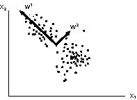
The set of values y^k = w^k x^T are called principal components of x.   The set of directions w are the principal directions in the sample space x for the variance y.   The variance y forms a high dimensional "ellipsoid": (assume <y>=0)

        <y²> = w C w^T

the direction w¹ corresponds to the direction of largest variation with variance l¹.  w² gives the second largest variance in a direction that is perpendicular to  w², w³ is third largest variation direction that is perpendicular to w¹ and w², and so on.  Here is in this plot a schematic illustration of the concept. 

What is good use of the above learning algorithm?  Such network can be used as a pre-processing layer in a multi-layer network for data reduction.  This will make the whole network faster (in learning).   In such applications,  the number N of input signals will be much larger than output signals M.  the mapping y = W x can be viewed as a form of data compression.

One particular interesting application is image data compression.  Since the set of w's form a new orthogonal axis, we can expand any arbitrary input data x along these axis,

        x = b₁ w¹ + b₂ w² + b₃ w³ + ...

multiplying (scale product with) w^k to both side of the equation, we find

        b_k = w^k x^T = y^k

In order to go back to x from b's without loss of information, we need N components of b.  However, if we keep only the first M components, then they represent a compressed information.  We test this idea with the example of Mathematica code.