8 Centre of Mass Frame*
\[ \newcommand\v[1]{\boldsymbol{#1}} \newcommand\vdot[2]{\v{#1}\cdot\v{#2}} \]
\[ \newcommand{\dd}[2][]{\mathrm{d}^{#1}#2} \]
\[ \newcommand\f[2]{\dfrac{#1}{#2}} \newcommand\da[2]{\dfrac{d #1}{d #2}} \newcommand\daa[2]{\dfrac{d^2 #1}{d #2^2}} \newcommand\pa[2]{\dfrac{\partial #1}{\partial #2}} \newcommand\pal[3]{\left.\dfrac{\partial #1}{\partial #2}\right|_{#3}} \newcommand\paa[2]{\dfrac{\partial^2 #1}{\partial #2^2}} \newcommand\pab[3]{\dfrac{\partial^2 #1}{\partial #2 \partial #3}} \def\half{\frac{1}{2}} \]
\[ \newcommand\ket[1]{\left|#1\right\rangle} % |x> \newcommand\exp[1]{\left\langle#1\right\rangle} % <x> \newcommand\lr[1]{\left(#1\right)} % (x) \newcommand\lrs[1]{\left[#1\right]} % [x] \newcommand\lra[1]{\left|#1\right|} % |x| \newcommand\lrc[1]{\left\{#1\right\}} % {x} \newcommand\lrl[3]{\left.#1\right|_{#2}^{#3}} % x_limits \]
\[ \def\ie{\text{i.e.}\quad} \]
\[ \newcommand{\me}[3][\rightarrow]{{#2}#1{#3}} % Typical reaction \newcommand{\nr}[3]{{#1}\,({#2})\,{#3}} % Nuclear reactions \newcommand{\ele}[4]{_{#2}^{#3}{\textbf{#1}}_{#4}} \newcommand{\el}[2]{^{#2}\text{#1}} \newcommand{\til}[2][\mathbf{\sim}]{\underset{#1}{{#2}}} \newcommand{\b}[1]{\overline{#1}} \]
\[ \newcommand{\coulomb}[1]{\dfrac{#1}{4\pi\epsilon_0}} \def\degree{^*} \]
\[ \def\amu{\text{ amu}} \def\J{\text{ J}} \def\K{\text{ K}} \def\s{\text{ s}} \def\second{\text{ s}} \def\Psecond{\text{ s}^{-1}} \def\m{\text{ m}} \def\mm{\text{ mm}} \def\km{\text{ km}} \def\fm{\text{ fm}} \def\mum{\text{ $\mu$m}} \def\mus{\text{ $\mu$s}} \def\mPERs{\text{ ms$^{-1}$}} \def\eV{\text{ eV}} \def\keV{\text{ keV}} \def\GeV{\text{ GeV}} \def\MeV{\text{ MeV}} \def\MeVc{\text{ MeV/c$^2$}} \def\KeVc{\text{ KeV/c$^2$}} \newcommand\ttp[1]{\times 10^{#1}} % To The Power \]
\[ \def\en{\nu_e} \def\Aen{\b{\nu_e}} \def\mun{\nu_\mu} \def\Amun{\b{\nu}_\mu} \]
\[ \def\uraniumA{\ele{U}{92}{233}{}} \def\uraniumB{\ele{U}{92}{235}{}} \def\uraniumC{\ele{U}{92}{238}{}} \def\carbonB{\ele{C}{6}{14}{}} \def\nitrogenB{\ele{N}{7}{14}{}} \def\oxygenA{\ele{O}{8}{14}{}} \def\oxygenB{\ele{O}{8}{16}{}} \]
\[ % \def\com{\text{\scriptsize CM}} \def\com{\mathrm{\scriptsize CM}} \]
\[ \def\l{l} \]
\[ \def\g{\gamma} \]
What to Expect in This Chapter
By now, you will have realised the importance of the centre-of-mass frame. This short chapter will bring together the basic ideas we need and establish the relationship between scattering angles measured in the centre-of-mass and laboratory frames.
Our treatment here is mostly non-relativistic and applies to a two-body elastic collision because these will be what we typically encounter. We will need these results later when we discuss scattering cross-sections.
8.1 The Centre-of-Mass Frame
The laboratory frame, or LAB frame, is the frame in which the target is initially at rest. The centre-of-mass frame, or CM frame, moves with the centre of mass. The CM frame is also called the zero-momentum frame. You will shortly see why.
Consider a projectile of mass \(m_1\) moving with initial velocity \(\v{u}_0\):
\[ \v{u}_1=\v{u}_0, \]
towards a target of mass \(m_2\) that is initially at rest:
\[ \v{u}_2=0. \]
As is usual when describing collisions, we take the incident beam direction as our reference direction. I will also use \(u_0=|\v{u}_0|\) to denote the speed associated with the velocity vector \(\v{u}_0\).
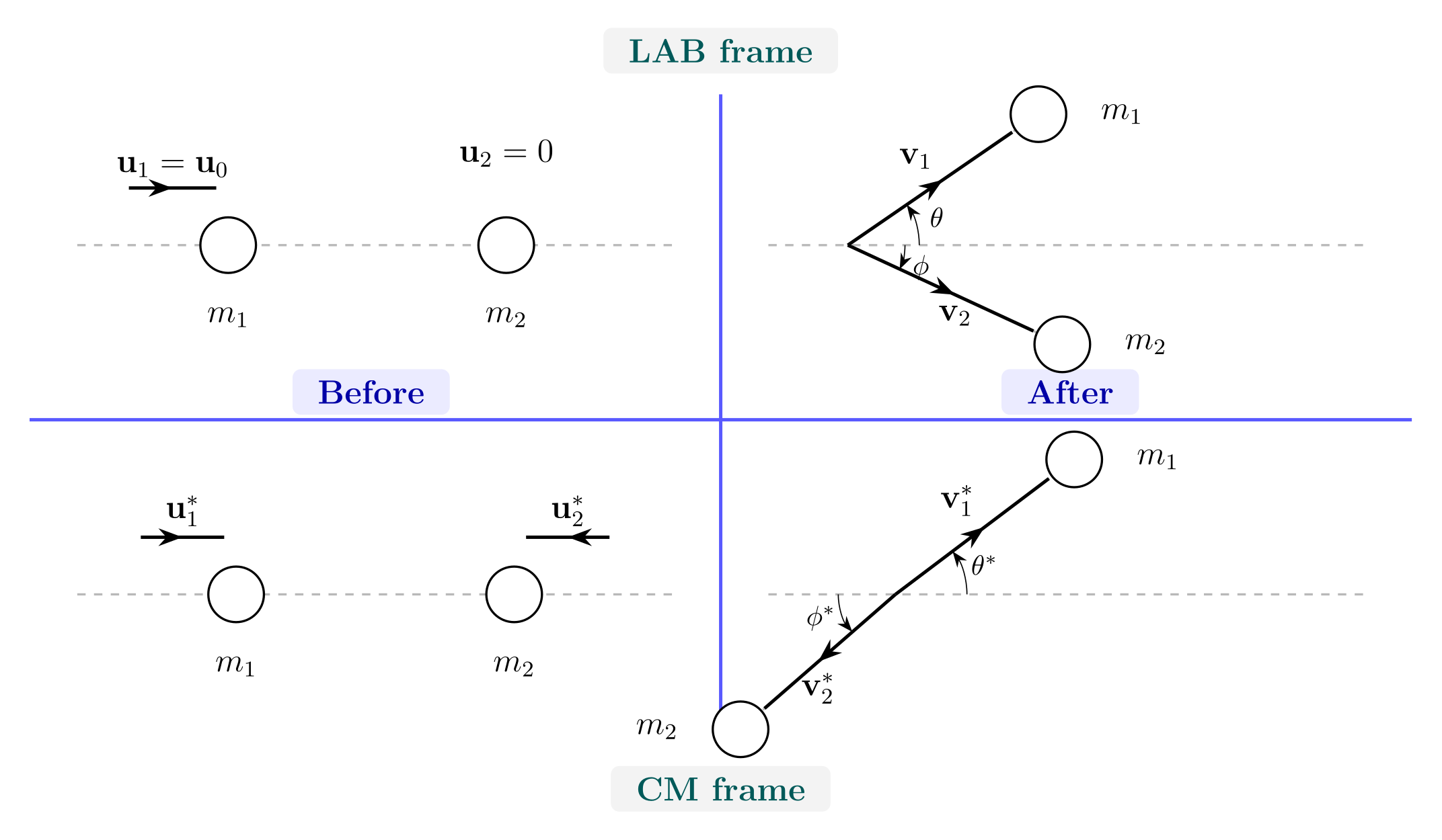
Note that in Figure 8.1, I have used the notation:
- \(\v u_i\) and \(\v v_i\) for velocities before and after the collision in the LAB frame;
- \(\v u_i^*\) and \(\v v_i^*\) for the corresponding velocities in the CM frame; and
- \(\v{u}_\com\) for the velocity of the CM frame relative to the lab.
8.2 Locating the Centre of
The location of the CM of a system of particles is defined as: \[ \v r_{\mathrm{CM}} = \f{\sum m_i\v r_i}{\sum m_i}. \tag{8.1}\]
For two particles, this reduces to:
\[ \v r_{\mathrm{CM}} = \frac{m_1\v r_1+m_2\v r_2} {m_1+m_2}. \tag{8.2}\]
Differentiating with respect to time gives the velocity of the centre of mass:
\[ \v u_{\mathrm{CM}} = \frac{m_1\v u_1+m_2\v u_2} {m_1+m_2}. \tag{8.3}\]
Since the target is initially at rest,
\[ \v u_{\mathrm{CM}} = \frac{m_1}{m_1+m_2}\v u_0. \tag{8.4}\]
It is often convenient to introduce the reduced mass,
\[ \mu = \frac{m_1m_2}{m_1+m_2}. \tag{8.5}\]
so that Equation 8.4 becomes
\[ \v u_{\mathrm{CM}} = \frac{\mu}{m_2}\v u_0. \tag{8.6}\]
8.3 Transforming to the CM Frame
In non-relativistic mechanics, velocities in the CM frame are obtained by the1 transformation:
1 Galilean
\[ \mathbf u_i^* = \mathbf u_i-\mathbf u_{\mathrm{CM}}. \tag{8.7}\]
For the projectile,
\[ \begin{aligned} \mathbf u_1^* &= \mathbf u_0 - \frac{m_1}{m_1+m_2}\mathbf u_0\\ &= \frac{m_2}{m_1+m_2}\mathbf u_0\\ &= \frac{\mu}{m_1}\mathbf u_0. \end{aligned} \tag{8.8}\]
For the target,
\[ \begin{aligned} \mathbf u_2^* &= -\mathbf u_{\mathrm{CM}}\\ &= -\frac{m_1}{m_1+m_2}\mathbf u_0\\ &= -\frac{\mu}{m_2}\mathbf u_0. \end{aligned} \tag{8.9}\]
The two particles therefore approach one another from opposite directions in the CM frame.
8.4 Zero Total Momentum
Let us verify that the total momentum is zero in the CM frame.
Before the collision: \[ \begin{aligned} \mathbf P_{\mathrm{total}}^* &= m_1\mathbf u_1^*+m_2\mathbf u_2^*\\ &= m_1\left(\frac{\mu}{m_1}\mathbf u_0\right) - m_2\left(\frac{\mu}{m_2}\mathbf u_0\right)\\ &=\v 0. \end{aligned} \tag{8.10}\]
Momentum is conserved, so the total momentum after the collision must also be zero:
\[ m_1\mathbf v_1^*+m_2\mathbf v_2^*=0. \tag{8.11}\]
Therefore,
\[ m_1\mathbf v_1^* = -m_2\mathbf v_2^*. \tag{8.12}\]
The two particles leave the collision with equal and opposite momenta. Their velocity vectors therefore point in diametrically opposite directions.
8.5 No Change in the CM Speeds
For a two-body elastic collision, the interaction changes the directions of the particles in the CM frame but not their individual speeds.
Since the total momentum is zero, before and after the collison:
\[ m_1u_1^*=m_2u_2^*, \tag{8.13}\]
and \[ m_1v_1^*=m_2v_2^*. \tag{8.14}\]
Hence,
\[ u_2^*=\frac{m_1}{m_2}u_1^*, \qquad v_2^*=\frac{m_1}{m_2}v_1^*. \tag{8.15}\]
Since the collision is elastic, kinetic energy is also conserved:
\[ \frac12m_1(u_1^*)^2+ \frac12m_2(u_2^*)^2 = \frac12m_1(v_1^*)^2+ \frac12m_2(v_2^*)^2. \tag{8.16}\]
Substituting the momentum relations gives
\[ \frac12m_1 \left(1+\frac{m_1}{m_2}\right)(u_1^*)^2 = \frac12m_1 \left(1+\frac{m_1}{m_2}\right)(v_1^*)^2. \]
Therefore,
\[ u_1^*=v_1^*. \tag{8.17}\]
The same reasoning gives
\[ u_2^*=v_2^*. \tag{8.18}\]
Thus, in the CM frame, an elastic two-body collision simply rotates the two velocity vectors while preserving their magnitudes.
8.6 Lab and CM Scattering Angles
As shown in Figure 8.1, \(\theta^*\) is the projectile’s scattering angle in the CM frame, while \(\theta\) is its scattering angle in the LAB frame. Both angles are measured relative to the projectile’s initial direction of motion.
The final projectile velocities in the two frames are related by
\[ \mathbf v_1 = \mathbf v_1^*+\mathbf u_{\mathrm{CM}}. \tag{8.19}\]
Resolving this vector equation into components gives
\[ v_1\cos\theta = v_1^*\cos\theta^*+u_{\mathrm{CM}} \tag{8.20}\]
and
\[ v_1\sin\theta = v_1^*\sin\theta^*. \tag{8.21}\]
Dividing the vertical component by the horizontal component gives
\[ \tan\theta = \frac{v_1^*\sin\theta^*} {v_1^*\cos\theta^*+u_{\mathrm{CM}}}. \]
Therefore,
\[ \tan\theta = \frac{\sin\theta^*} {\cos\theta^*+\zeta}, \tag{8.22}\]
where
\[ \zeta \equiv \frac{u_{\mathrm{CM}}}{v_1^*}. \tag{8.23}\]
Because the collision is elastic,
\[ v_1^*=u_1^*=\frac{\mu}{m_1}u_0. \]
Consequently,
\[ \zeta = \frac{(\mu/m_2)u_0}{(\mu/m_1)u_0} = \frac{m_1}{m_2}. \tag{8.24}\]
The relationship between the two scattering angles is therefore
\[ { \tan\theta = \frac{\sin\theta^*} {\cos\theta^*+m_1/m_2} }. \tag{8.25}\]
An alternative form, which will be useful when transforming cross-sections, is
\[ { \cos\theta = \frac{\cos\theta^*+\zeta} {\sqrt{1+2\zeta\cos\theta^*+\zeta^2}} }, \qquad \zeta=\frac{m_1}{m_2}. \tag{8.26}\]
8.7 Checking the Result
A useful formula should agree with our physical intuition in simple limiting cases.
8.7.1 A Very Heavy Target: \(m_2\gg m_1\)
In this limit, \[ \zeta=\frac{m_1}{m_2}\longrightarrow0, \] so \[ \tan\theta\longrightarrow\tan\theta^*. \] Therefore, \[ \theta\approx\theta^*. \]
The heavy target barely moves, so the lab and CM frames are almost the same.
8.7.2 Equal Masses: \(m_1=m_2\)
Here, \(\zeta=1\), and
\[ \tan\theta = \frac{\sin\theta^*}{1+\cos\theta^*} = \tan\left(\frac{\theta^*}{2}\right). \]
Thus,
\[ \theta=\frac{\theta^*}{2}. \]
This gives us an interesting insight. Since \(0\leq\theta^*\leq\pi,\) the LAB scattering angle satisfies \(0\leq\theta<\f{\pi}{2}\).
Thus, when \(m_1=m_2\), the projectile cannot scatter backwards in the LAB frame. Its LAB scattering angle approaches \(90^\circ\) as \(\theta^*\) approaches \(\pi\).
8.8 The Relativistic CM Frame
The ideas developed above are non-relativistic, but the defining property of the CM frame remains valid in relativistic mechanics: \[ \mathbf P_{\mathrm{total}}^*=0. \tag{8.27}\]
In relativistic particle physics, it is more precise to use the term centre-of-momentum frame, as it typically contains massless particles.
The important difference is that we can no longer transform velocities us Equation 8.7 by simply subtracting the velocity of the CM frame. Instead, it is usually easier to transform the total energy and momentum as a four-vector.
8.8.1 The Invariant Energy \(\sqrt{s}\)
For two incoming particles, consider the Lorentz invariant quantity \(s\) define as
\[ s = (E_1+E_2)^2 - c^2\left|\mathbf p_1+\mathbf p_2\right|^2. \tag{8.28}\]
In the CM frame, the total momentum is zero, so
\[ s=(E_1^*+E_2^*)^2. \]
Therefore,
\[ {\sqrt{s}=E_{\mathrm{CM}}}. \tag{8.29}\]
Thus, \(\sqrt{s}\) is the total energy available in the CM frame. Equivalently, \(\sqrt{s}/c^2\) is the invariant mass of the complete system.