By this point, you should possess a fundamental grasp of the quantum numbers and conservation laws associated with elementary particles. You should also have a sense of how we arrived at this understanding. In this chapter, I would like to discuss the dynamics of the various interactions in slightly greater depth. I will start by showing how to use Feynman diagrams to explore some of the mechanisms of particle interactions. Ultimately, you should have a satisfying (albeit non-mathematically) appreciation of how the four (well three) fundamental forces make the Universe work!
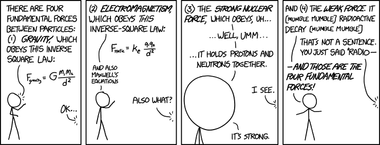
Hopefully you will not have any problem describing the four fundamental forces unlike in the comic below:
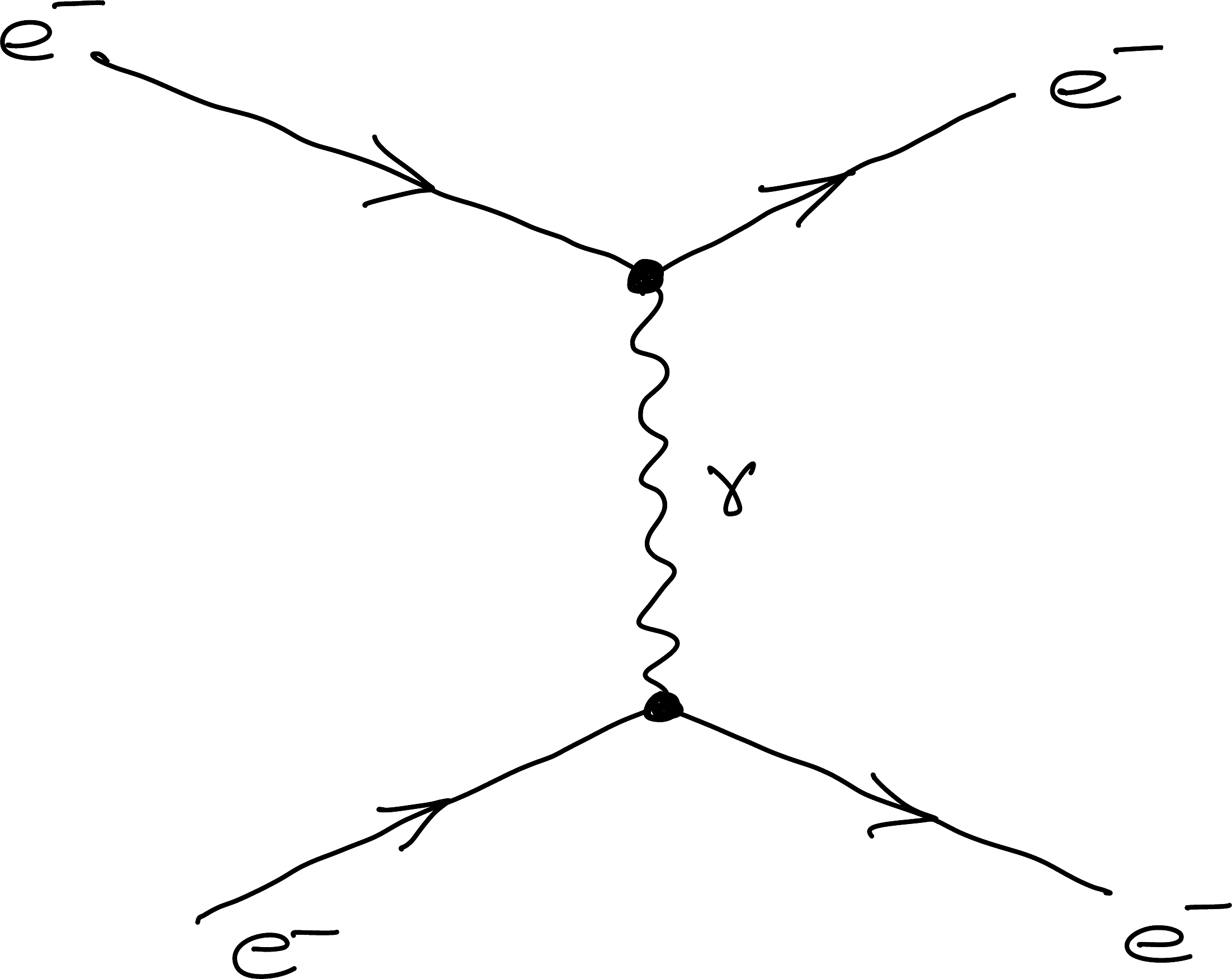
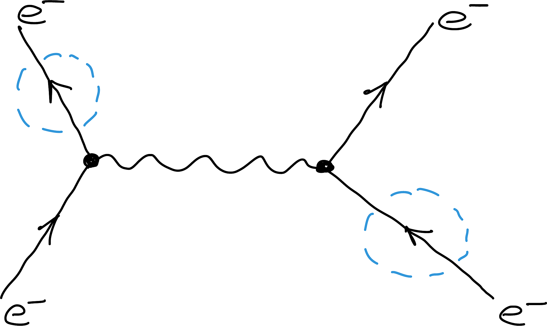
Figure 5.1 is a typical Feynman diagram. This diagram shows the interaction between two electrons mediated by a virtual photon.
Allow me to highlight the following features of Feynman diagrams:
Time flows from left to right.
You can make sense of this by imagining a vertical line scanning across the diagram.
The lines in the diagram are not trajectories.
The lines represent the particles’ states before and after the interaction.
For our purposes, they simply indicate what enters and leaves the central region.
The central region is never directly observed.
The central region shows details of the interaction, such as the exchange of the mediating particle—the virtual photon in this case. However, what happens in this region is never directly observed.
All Feynman diagrams are constructed by reusing primary vertices.
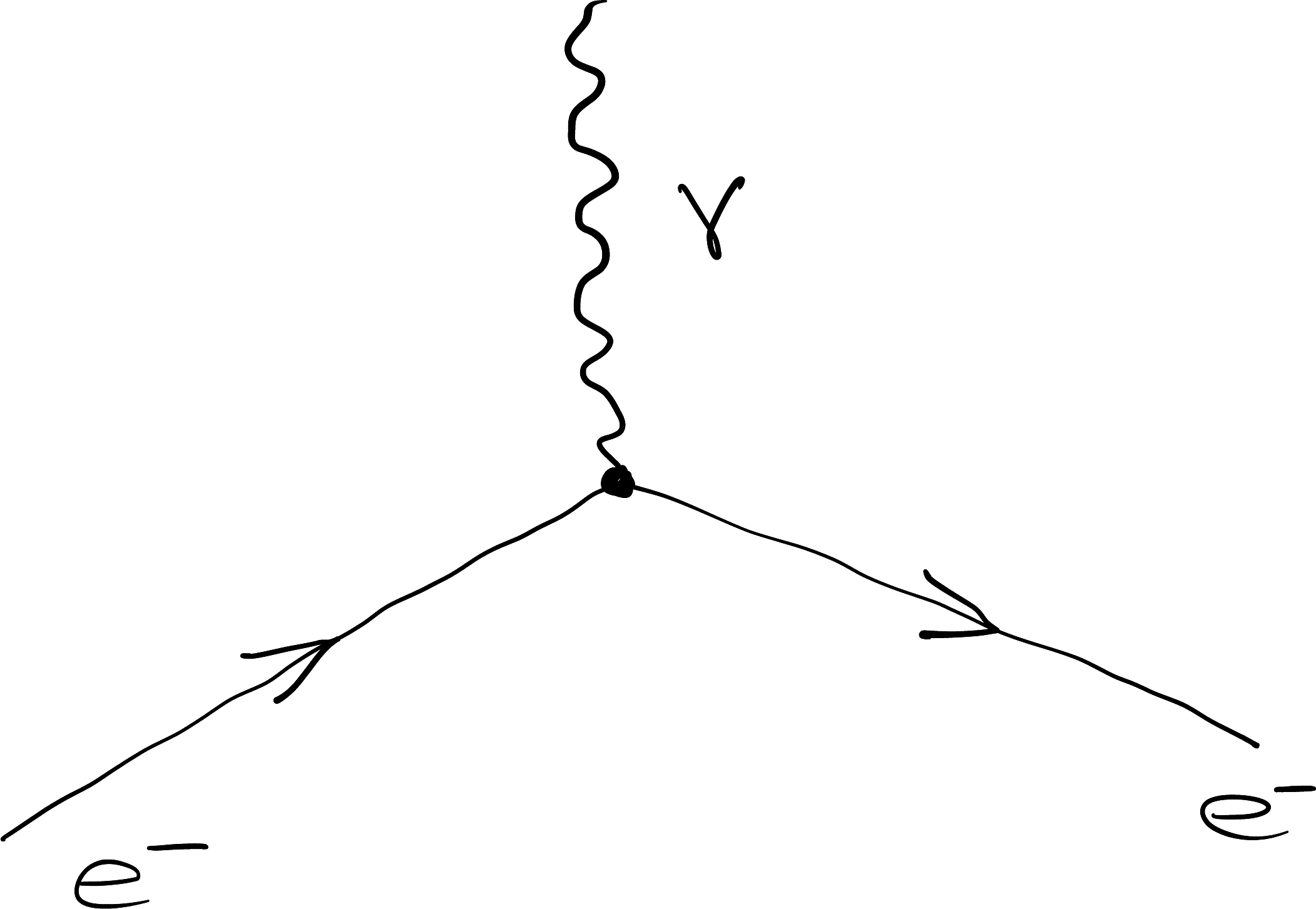
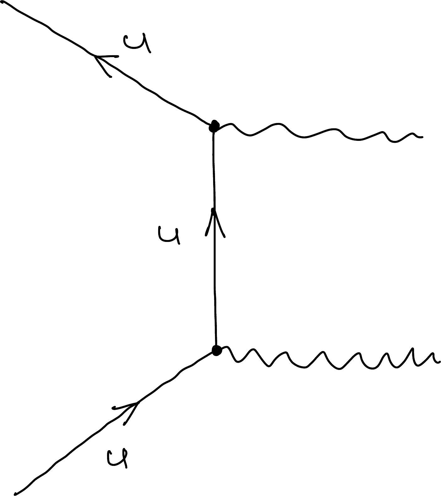
The primary vertex for the electromagnetic interaction is shown in Figure 5.2.
You cannot use this vertex on its own, as it does not represent a valid reaction:
\[
\me[\nrightarrow]{e}{e+\gamma}
\tag{5.1}\]
You need at least two such vertices to create a valid Feynman diagram. You can join primary vertices by matching photons or particles, taking care to preserve the directions of the arrows.
The arrows always pass through the vertex: one in and one out.
You should never have both arrows pointing into the vertex or both pointing out of it.
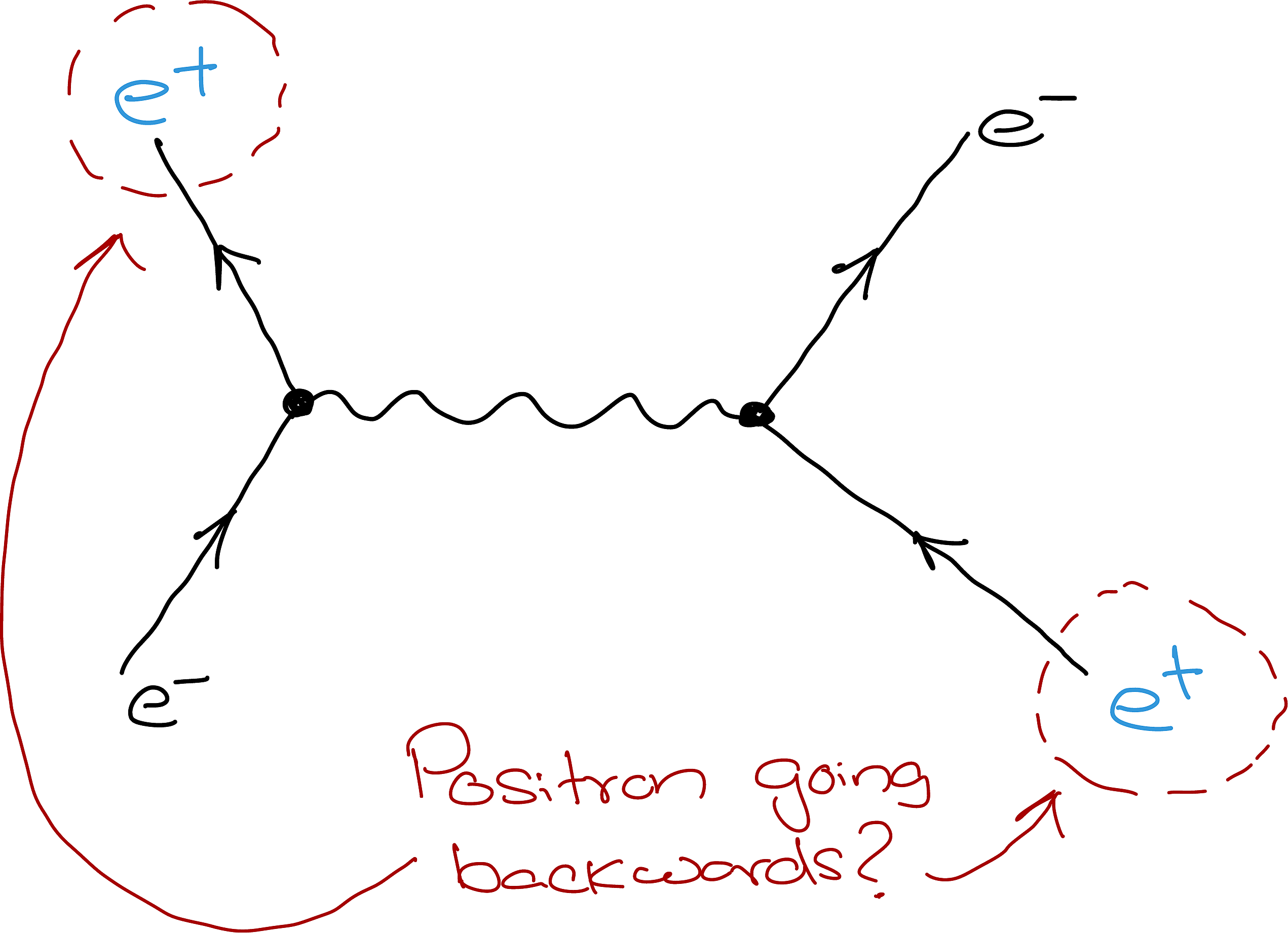
An arrow pointing opposite to the flow of time represents an antiparticle.
Figure 5.3 shows an electron at the bottom and a positron annihilating to produce a photon, which then produces a new electron–positron pair.
Be careful not to confuse others—or yourself—by mixing conventions.
WarningDon’t do this!
Don’t use \(e^+\) and \(e^-\) as it is confusing. The arrow already indicates this information.
Figure 5.1: Typical Feynman diagram showing two particles (two electrons in this case) interacting via a virtual particle (here a photon).
Figure 5.2: All Feynman diagrams are constructed by reusing a primary vertex like the one shown here. This is the primary vertex for an EM interaction.
Figure 5.3: Arrows always go through the vertex. Arrows going opposite to the flow of time correspond to antiparticles.
5.1.2 Twisting And Rotations Work Too!
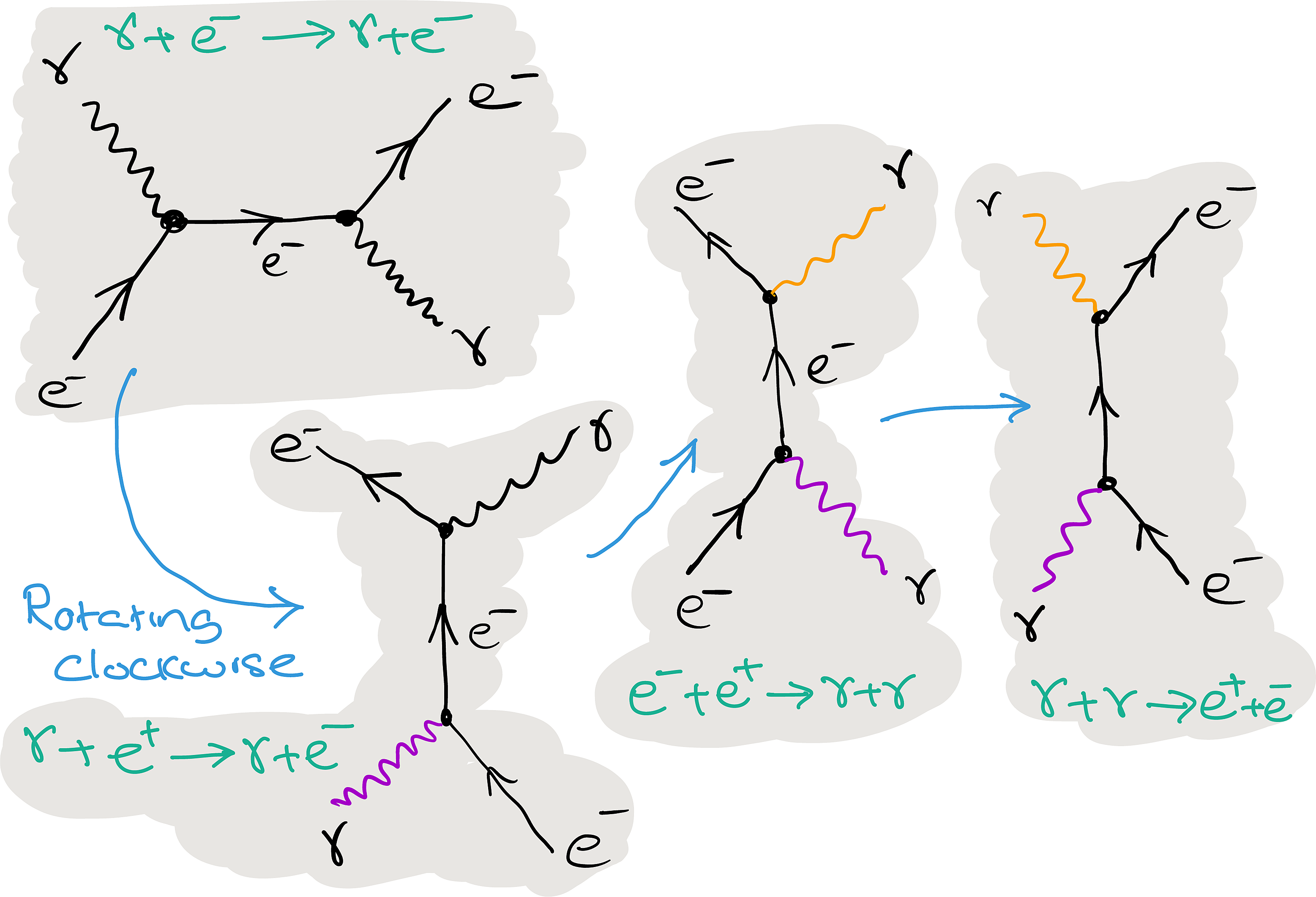
The principle of crossing symmetry is embodied in Feynman diagrams. Twisting or rotating a Feynman diagram can give another valid Feynman diagram corresponding to a different particle interaction, provided that no conservation law is violated. Consider Figure 5.4.
Figure 5.4: Compton scattering, electron–positron annihilation, and photon–photon pair production are related by crossing symmetry. Moving an ‘external’ line between the initial and final states replaces the particle with its antiparticle (I included the colours are for clarity; they don’t mean anything!).
Notice that, for the final pair-production process to take place, the total centre-of-momentum energy of the photons must be at least \(2m_e c^2\). This is a kinematic restriction that must be satisfied.
5.1.3 Multiple Vertices
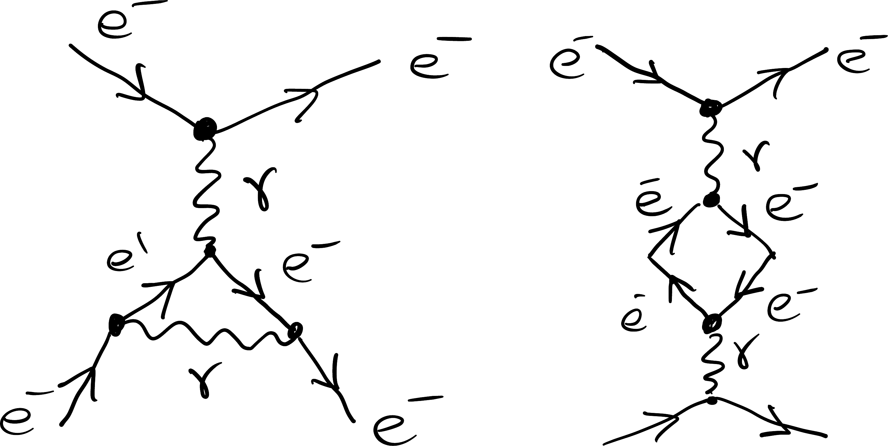
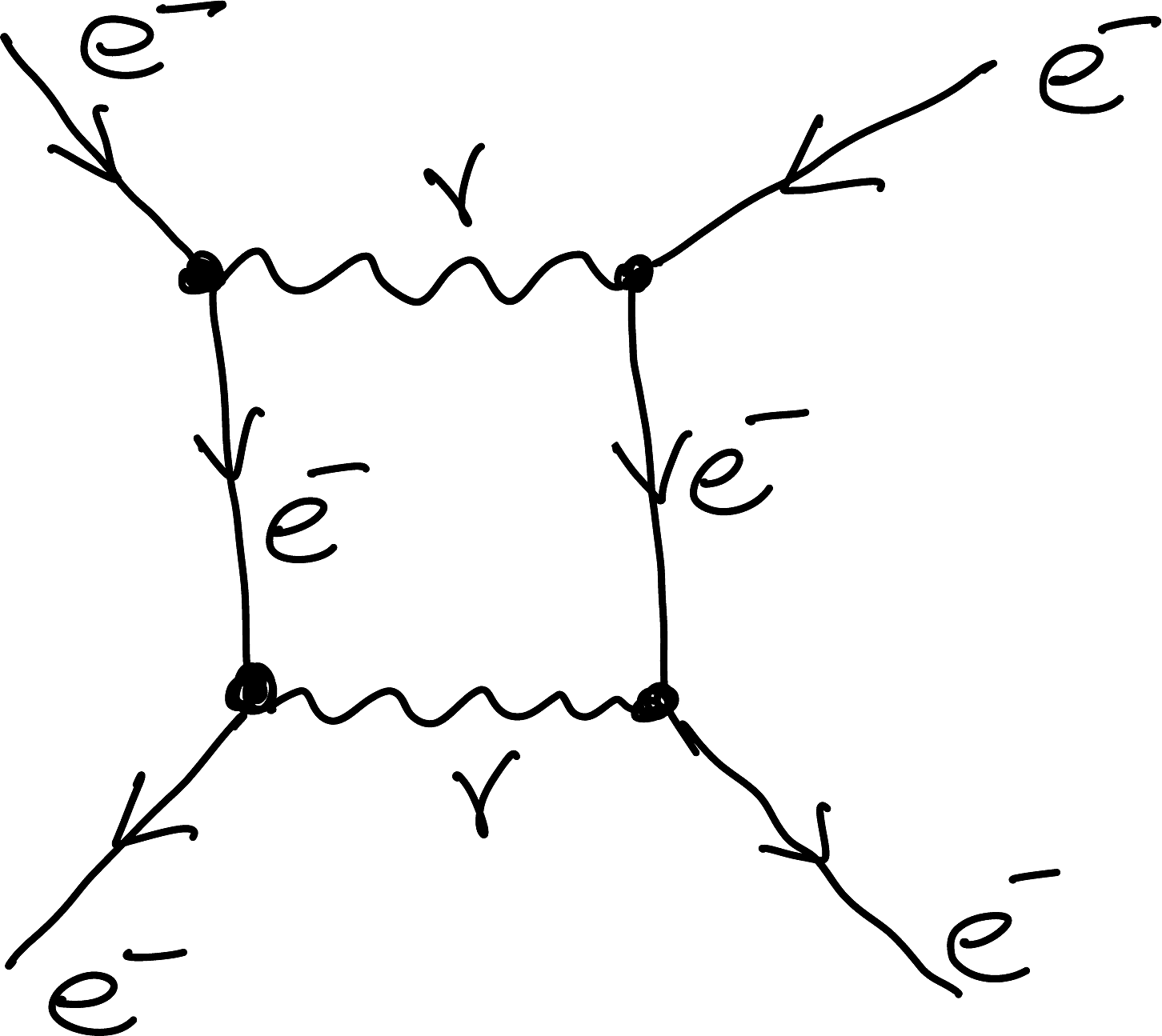
You can have more than one vertex. In fact, the point of the diagrams is to write out the multiple ways a process can occur. Here are some examples. What happens in the innards of the diagram does not matter (physically) as they are never observed. What does matter are the external lines. So for all the diagrams in Figure 5.5, two particles go in, and two particles come out.
Figure 5.5: Three examples of Feynman diagrams that have multiple vertices.
5.1.4 More Than Pretty Pictures
Feynman diagrams are more than pretty pictures. Using a set of rules called the Feynman rules, each diagram can be converted into a mathematical expression called an amplitude (this is beyond what we can do in this course. See here for an example from Wikipedia.). This amplitude indicates how much the process depicted by the diagram contributes to the transition in question. In the case of Figure 5.5, two electrons enter and two electrons leave.
We associate a dimensionless coupling strength with each vertex to make these diagrams quantitative. This coupling indicates how strongly the gauge boson interacts with the fermion.
For the electromagnetic interaction, the relevant measure of the coupling strength is the fine-structure constant, \(\alpha = \frac{1}{137}.\) The probability of an interaction is related to the number of vertices in the diagram. A diagram containing four electromagnetic vertices contributes at order \(\alpha^4\) to the probability.
We can draw an infinite number of increasingly complicated diagrams for the same process by adding more vertices. However, because \(\alpha\) is small, each additional level of complexity generally contributes much less to the overall process, at least in the case of the electromagnetic interaction.
5.2 Primary Interaction Vertices
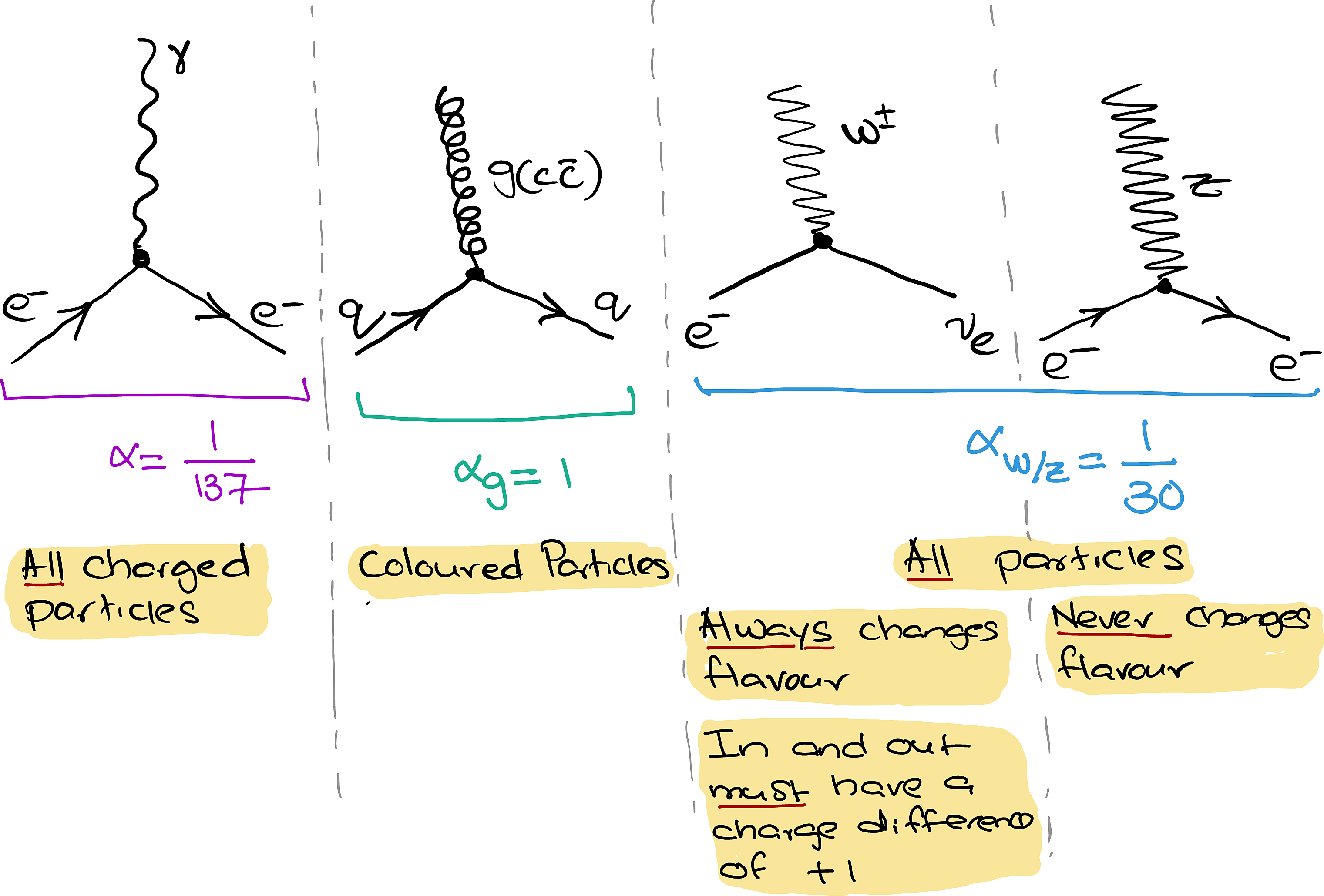
Our Universe works through the interactions of elementary particles via the four fundamental interactions. However, the different interactions do not couple with equal strength to every particle. More precisely, not all gauge bosons couple to all particles. The interactions of the various gauge bosons can be described using the interaction vertices of the Standard Model. These are shown below:
Figure 5.6: The interaction vertices of the Standard Model.
Take note of the following:
The electromagnetic interaction acts only on particles that carry electric charge. In other words, photons couple only to electrically charged particles.
The strong interaction acts only on particles that carry colour charge. In other words, gluons couple to particles carrying colour charge.
The weak interaction couples to all quarks and leptons, including neutrinos.
Coupling to a \(W^\pm\)always changes the flavour of a particle. This is accompanied by a change in electric charge of one unit (\(\pm1\)) between the incoming and outgoing particles.
The coupling constant for the weak interaction is larger than that for the electromagnetic interaction. However, the photon is massless, whereas the \(W^\pm\) and \(Z^0\) bosons are massive. At low energies, their large masses strongly suppress weak processes, making the weak interaction appear weaker than the electromagnetic interaction.
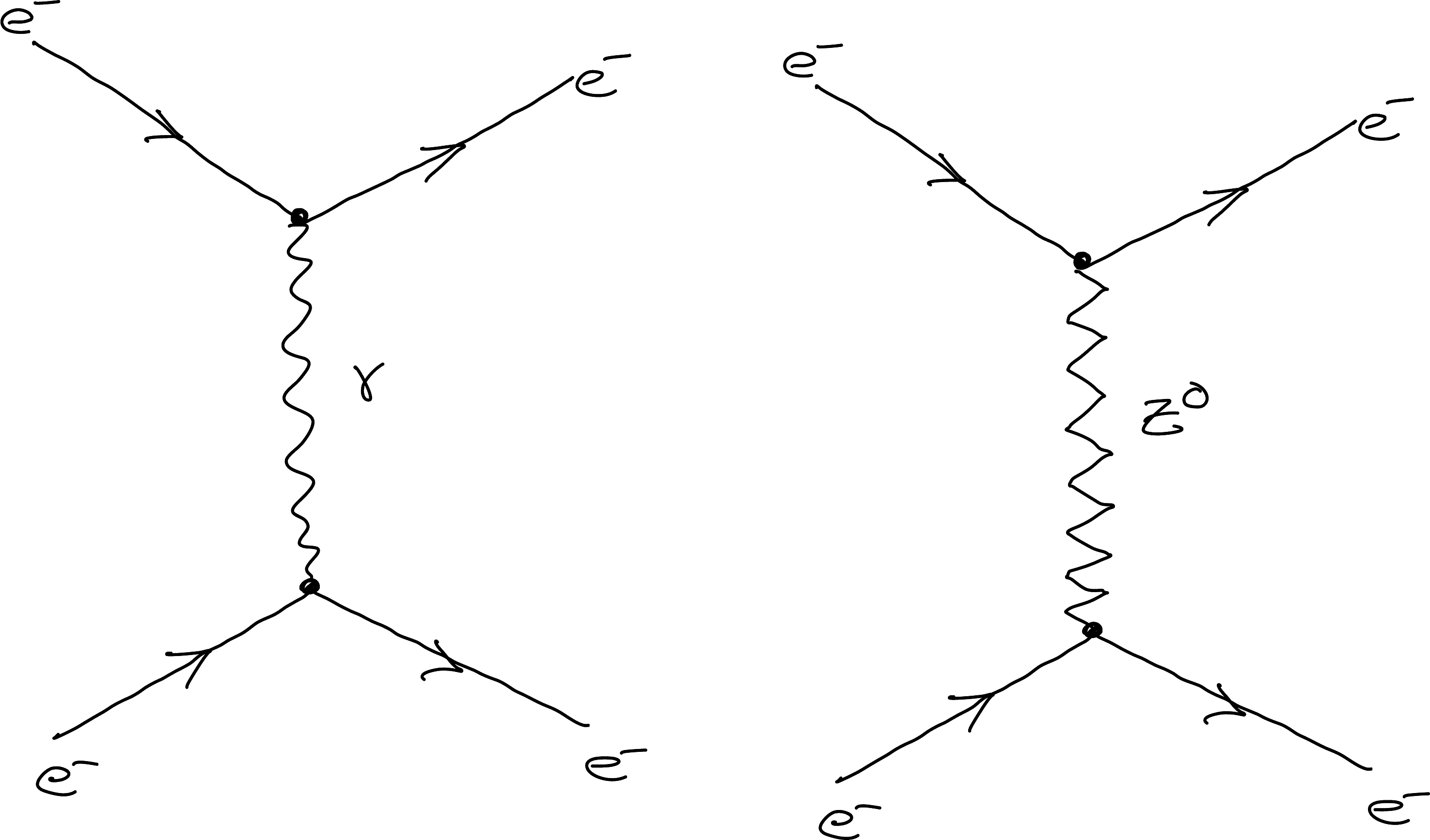
Notice the similarity between the electromagnetic interaction and the neutral weak interaction:
Figure 5.7: A neutral weak contribution to a predominantly electromagnetic process.
The latter provides a possible competing mechanism in processes involving charged particles, as shown below. This neutral weak contribution (sometimes referred to as neutral weak contamination) to the otherwise predominantly electromagnetic phenomena has been experimentally verified.
5.2.1 Conservation & the primary vertices
Every allowed interaction must obey the relevant conservation laws. We can use the primary vertices to see how quantities such as electric charge, colour charge, baryon number, and lepton number are conserved and how particle flavour may change.
Charge All three vertices enforce charge conservation. Even during a charged weak interaction, the gauge boson (\(W^\pm\)) carries away the charge allowing particles to change charge.
Baryon number You can say that baryons have a quark number of 3, and mesons have a quark number of 0. You will notice that for all the vertices if a quark goes in, a quark comes out. So, the baryon number is always conserved. However, this is not the case for mesons because they start with ‘zero’ net quarks.
Flavour The weak interaction can couple quarks between generations. So, for example, it is possible for strangeness to disappear because of a \(s\rightarrow u\) coupling. Therefore, in general, flavour is not conserved. However, if you stay away from the weak force, flavour can be ‘approximately’ conserved.
Lepton number Since the strong interaction does not affect leptons, we need only consider the other two interactions. For the electromagnetic interaction, the particle that goes in always comes out. For the weak interaction, too, if a lepton goes in, a lepton will always come out, although it might not be the same one! So, the lepton number is conserved.
Colour
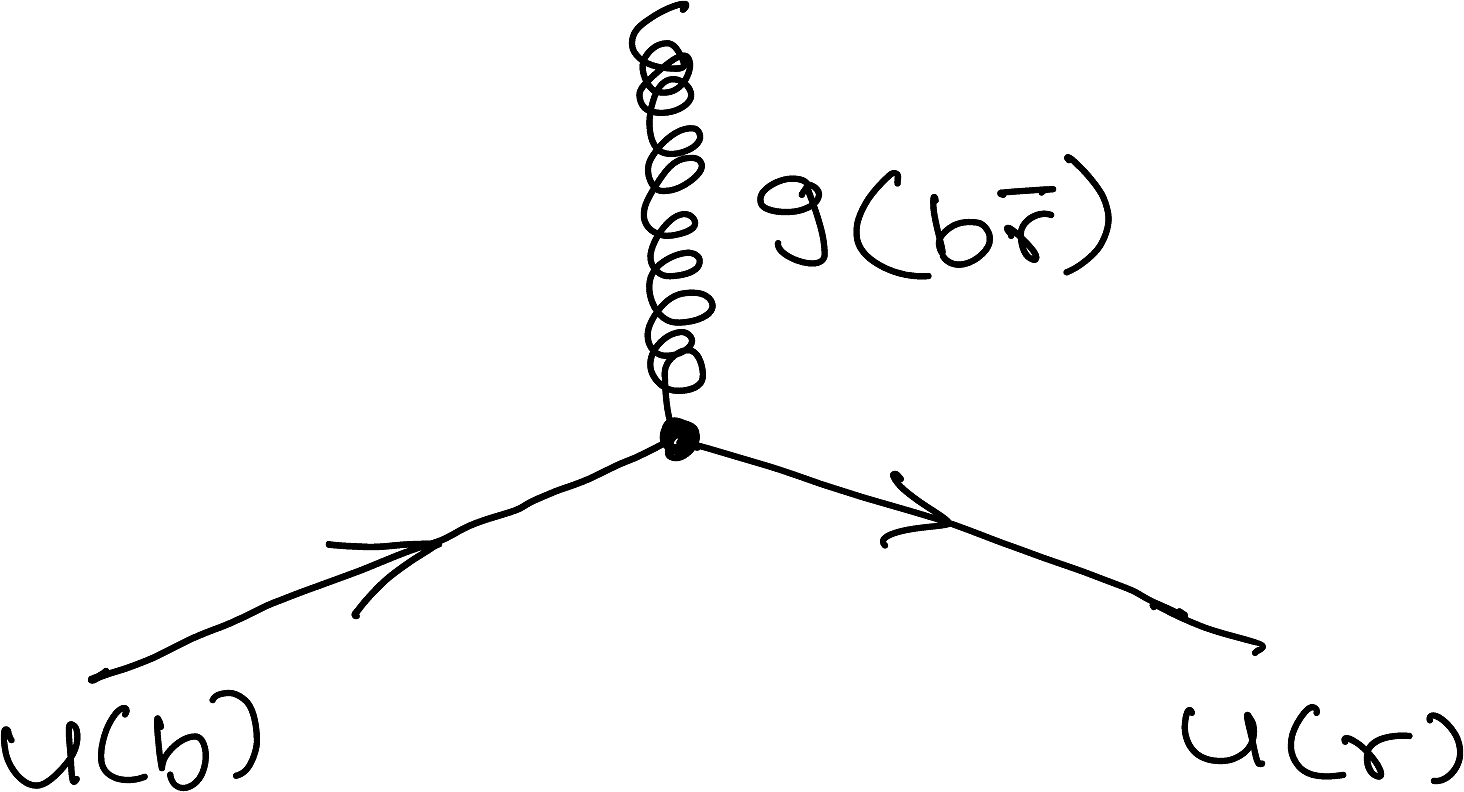
I must mention that the primary vertex for the strong interaction allows a gluon to change the colour of a quark. This is possible because the gluon carries a colour–anticolour combination, \(C\bar{C}\), ensuring that colour charge is conserved. A specific example is shown in Figure 5.8.
Figure 5.8: Colour can change during a strong interaction. The resulting change in colour is carried by the gluon.
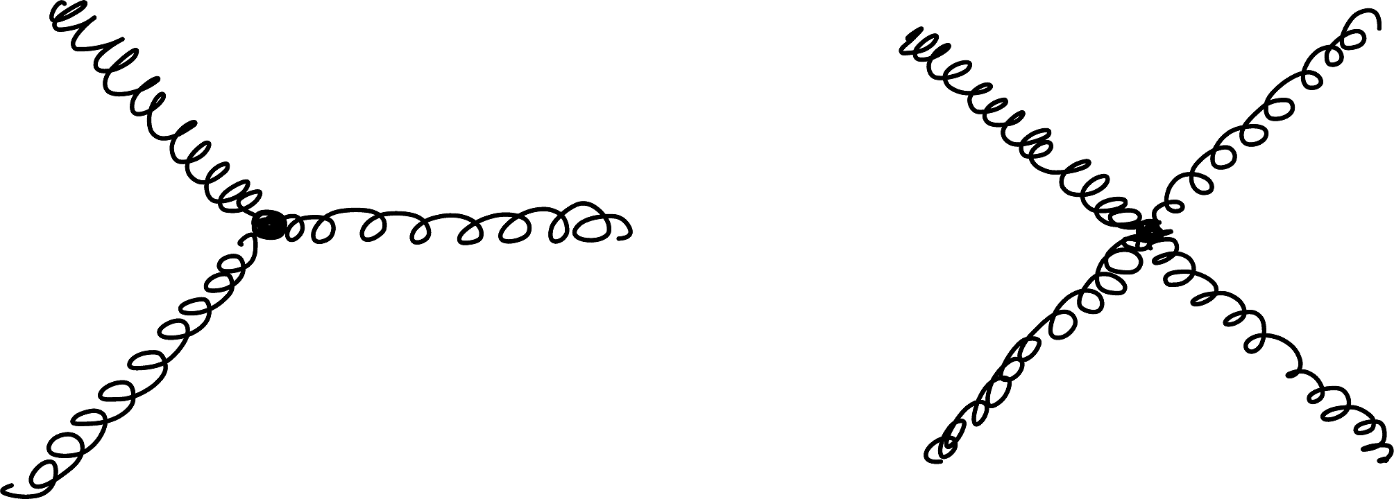
Figure 5.9: Gluons can also interact with other gluons.
Since gluons carry colour charge, they can also interact with other gluons. The strong interaction therefore has two additional primary interaction vertices, as shown in Figure 5.9. These vertices make the strong interaction richer (and more complicated) allowing possibilities such as the formation of particles called glueballs.
5.3 The Extent of the Weak Interaction
Since the charged weak interaction involves a charged gauge boson, \(W^\pm\), its coupling must change the electric charge of a fermion by one unit. The \(W^\pm\) boson carries the corresponding charge away from, or into, the vertex. Consequently, the charged weak interaction couples fermions whose electric charges differ by one unit.
The diagonal elements of the matrix are close to 1. Therefore, the charged weak interaction couples quarks within the same generation (for example, \(u\longleftrightarrow d\), \(c\longleftrightarrow s\), and \(t\longleftrightarrow b\)) more strongly than it couples quarks from different generations.
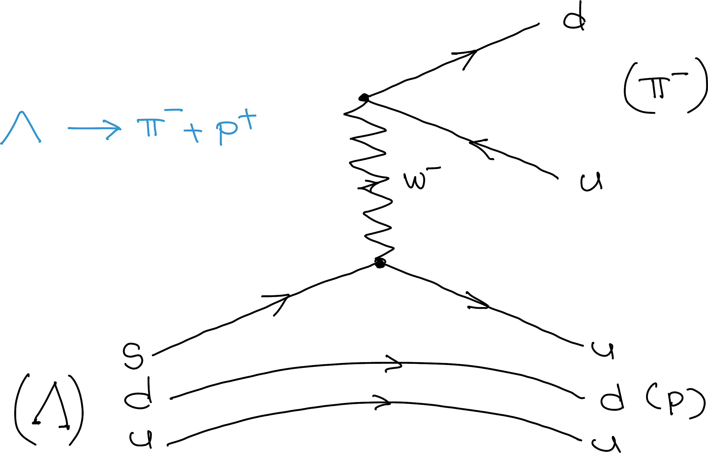
However, the non-zero off-diagonal elements mean that interactions between different generations can still occur. This is crucial: without these couplings, processes in which strangeness changes, such as
\[
\me{\Lambda}{p+\pi^-},
\tag{5.7}\]
would not be possible.
5.4 Examples
Let me take you through several representative Feynman diagrams for different particle interactions. These examples will help you develop an intuition for what we mean by an interaction and build useful mental pictures of how particle interactions work.
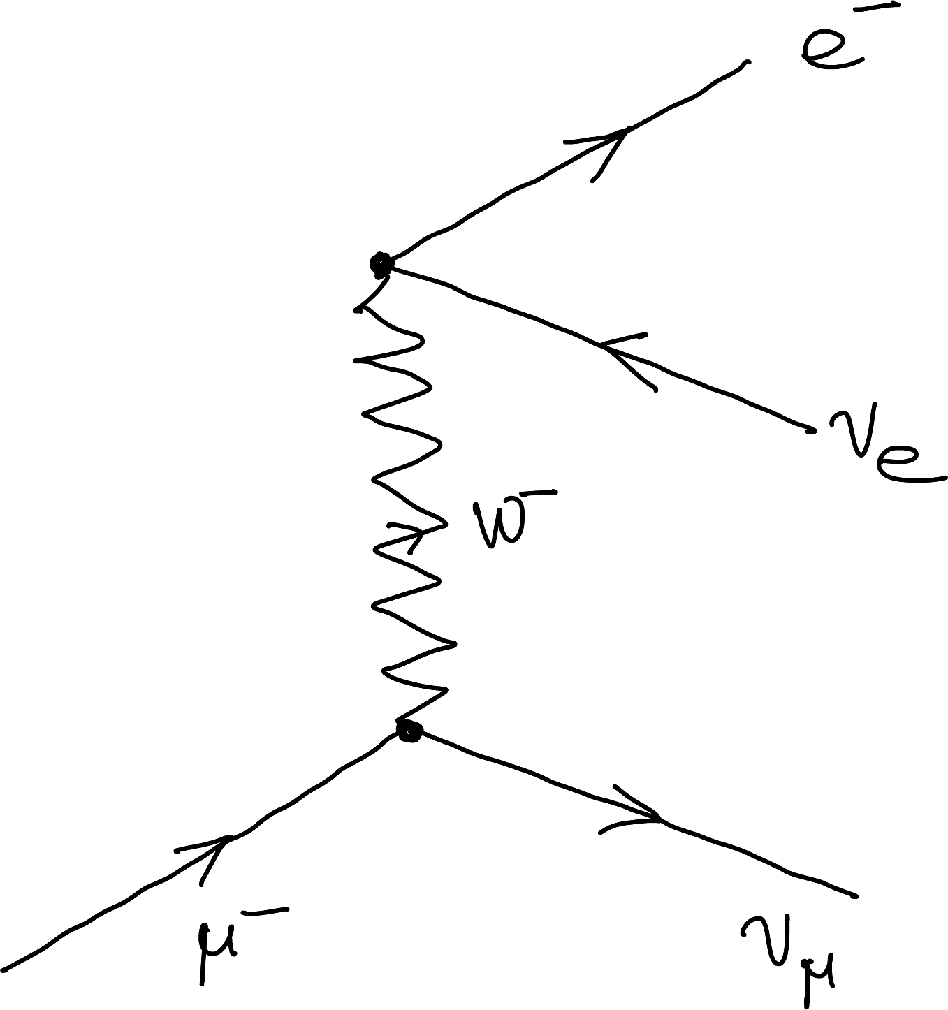
5.4.1 A Purely Leptonic Process: \(\mu\) decay
\[
\me{\mu^-}{e^-+\Aen+\mun}
\tag{5.8}\]
Figure 5.10
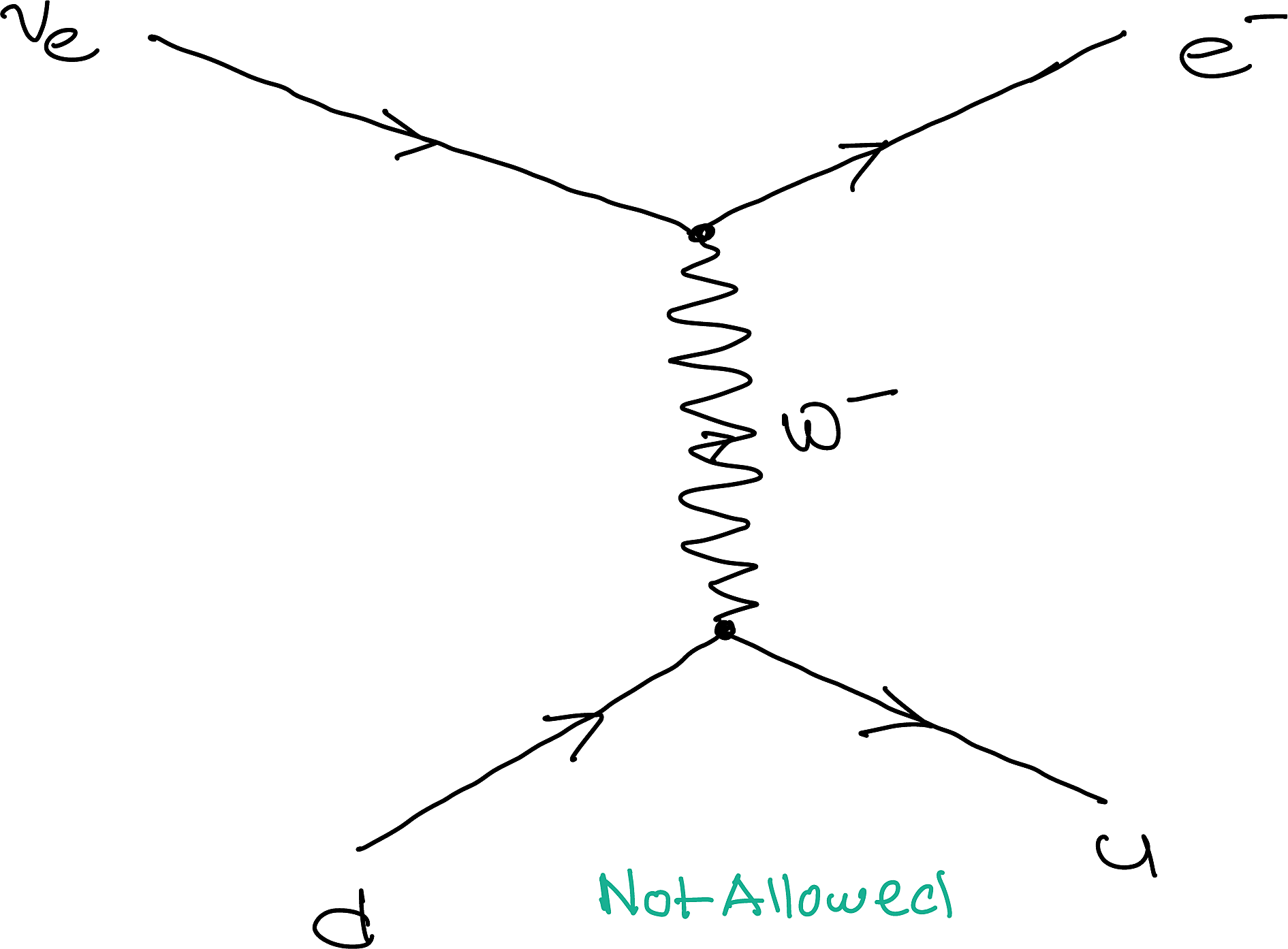
5.4.2 A Semileptonic Process: Changing \(d\) to \(u\)
Figure 5.11
A semileptonic process involves both quarks (or hadrons) and leptons.
The diagram represents the quark-level transition \(d\rightarrow u\). However, it cannot occur as a reaction involving free quarks because of quark confinement: isolated quarks are never observed. Instead, this transition must occur within a hadron.
We can “flip” the diagram to obtain a physically observable process, as shown in the next example.
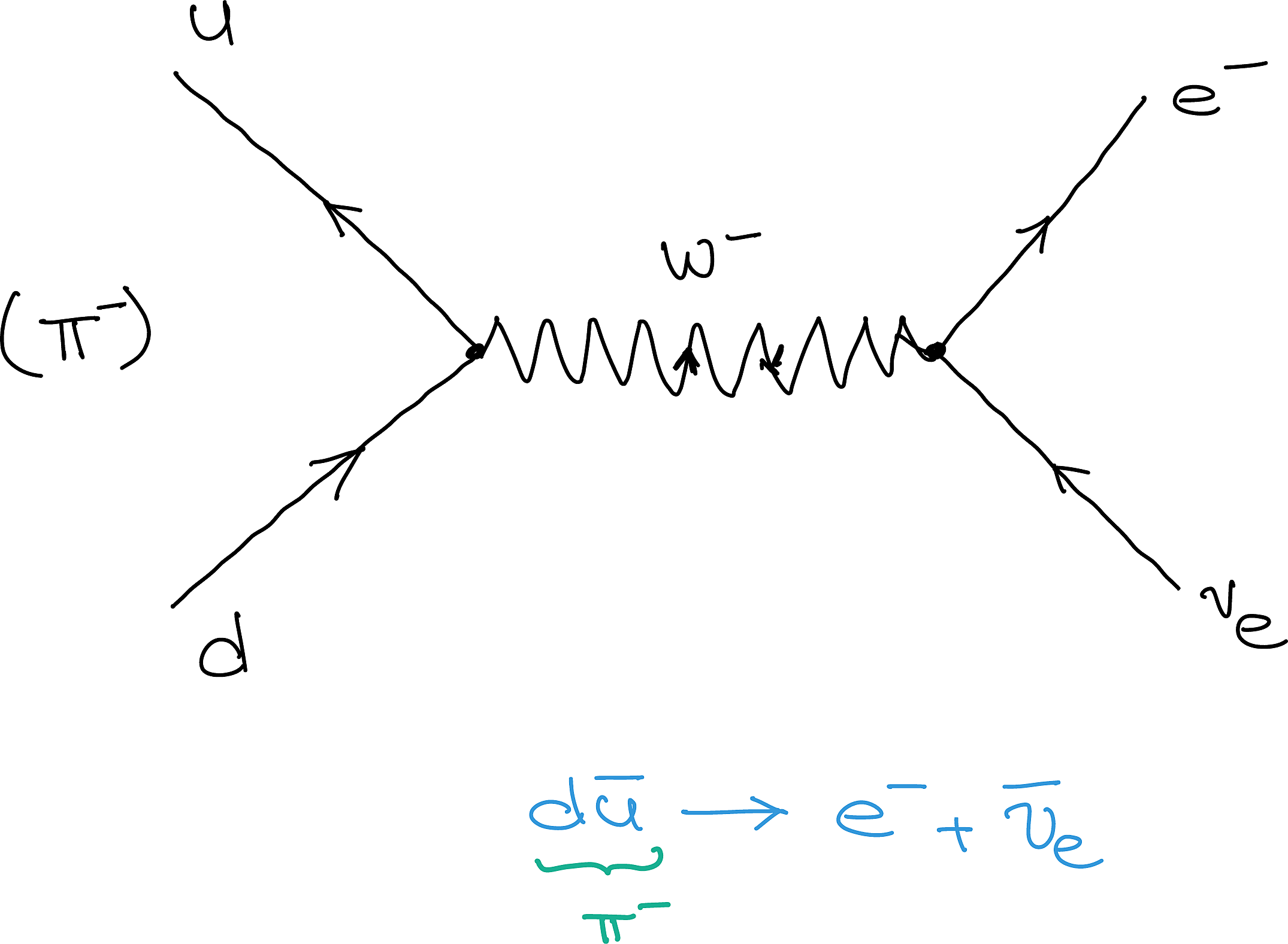
5.4.3 Decay Of \(\pi^-\)
\[
\me{\pi^-}{e^-+\Aen}
\tag{5.9}\]
Figure 5.12
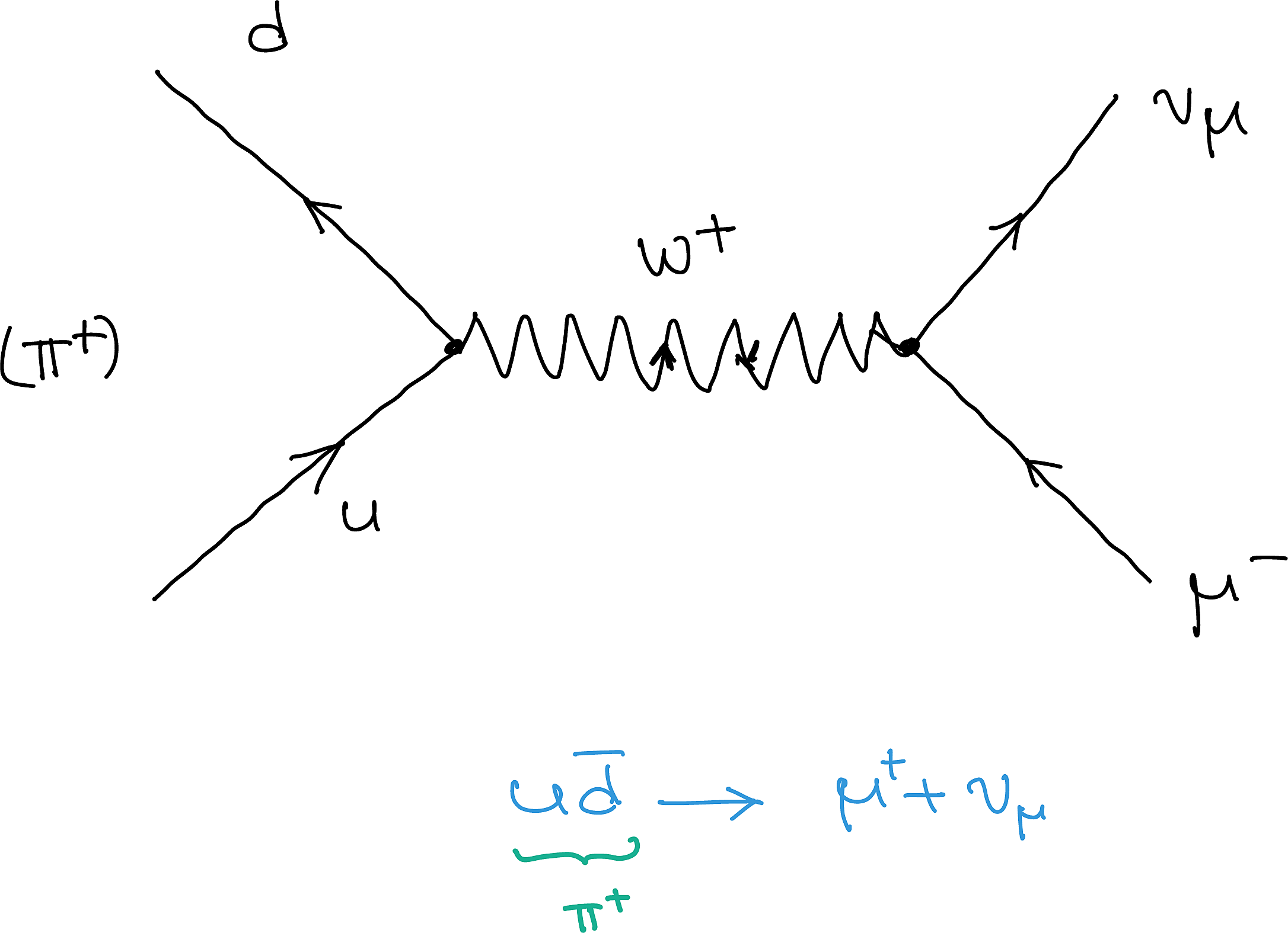
5.4.4 Decay Of \(\pi^+\)
\[
\me{\pi^+}{e^-+\en}
\tag{5.10}\]
Figure 5.13
5.4.5\(u/\b{u}\) Pair Annihilation
At first glance, the diagram shows a \(u\bar{u}\) pair annihilating through the electromagnetic interaction.
Because of quark confinement, however, this process is not observed with individual free quarks. The incoming \(u\bar{u}\) pair can instead be understood as a bound component of a neutral pion. In this light, the diagram represents \[
\me{\pi^0}{\gamma+\gamma}.
\tag{5.11}\]
So, the decay of the \(\pi^0\) can be understood at the quark level as quark–antiquark annihilation through the electromagnetic interaction. This helps explain why the \(\pi^0\) decay is about nine orders of magnitude faster than the weak decay of the charged pion: \[
\me{\pi^+}{\mu^+ + \nu_\mu}.
\tag{5.12}\]
The latter reaction must “hang around” much longer before the weak interaction works its magic. You saw the Feynman diagram for a similar decay in Figure 5.13.
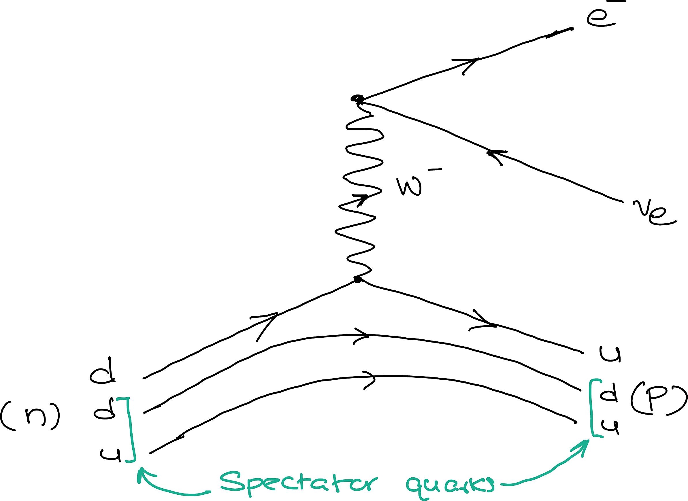
5.4.6\(\beta\)-decay of \(n\)
\[
\me{n}{p^+ +e^- + \Aen}
\tag{5.13}\]
Figure 5.14
Notice the two \(du\) quarks that come along for the ride as spectators due to being strongly bound together.
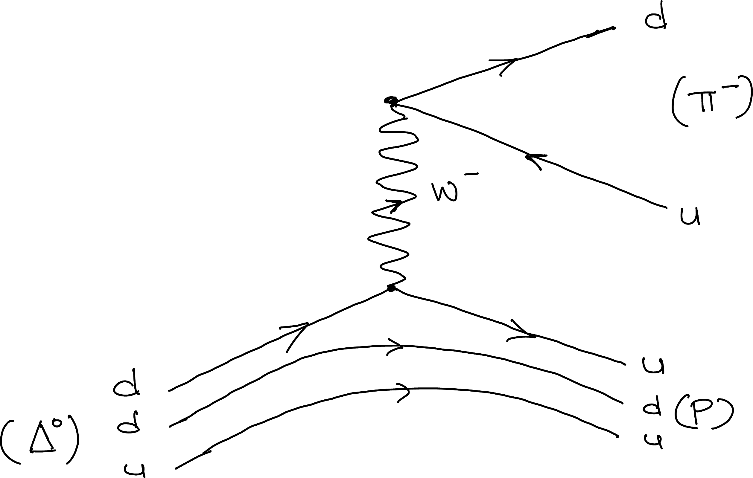
5.4.7 Weak Decay Of \(\Delta^0\)
\[
\me{\Delta^0}{p^+ +\pi^-}
\tag{5.14}\]
Figure 5.15
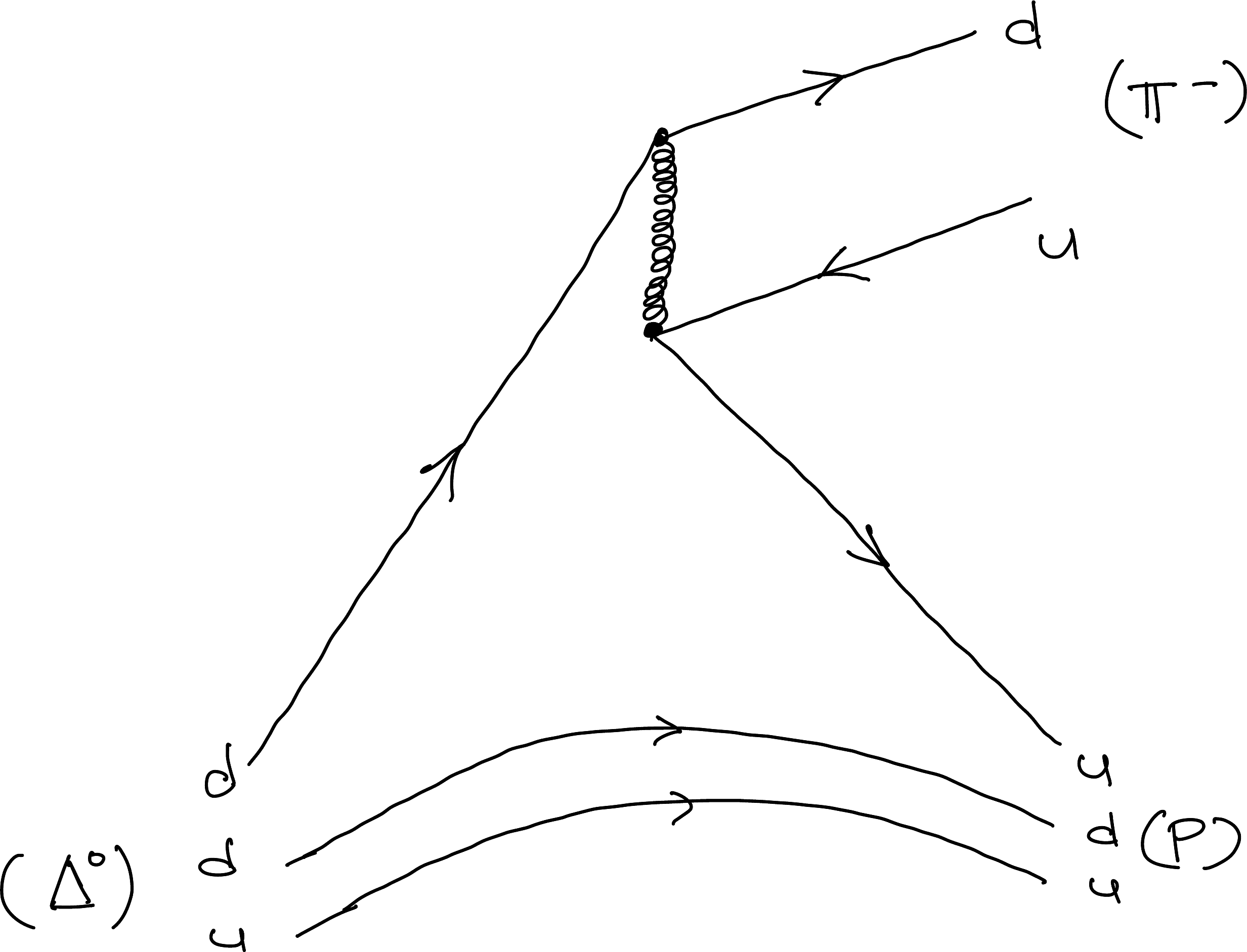
This charged weak decay must compete with the purely hadronic decay driven by the strong interaction shown in the next example. Consequently, this weak decay mode contributes only a very small fraction of the particle’s total decay rate.