12 Hello Nucleus
\[ \newcommand\v[1]{\boldsymbol{#1}} \newcommand\vdot[2]{\v{#1}\cdot\v{#2}} \]
\[ \newcommand{\dd}[2][]{\mathrm{d}^{#1}#2} \]
\[ \newcommand\f[2]{\dfrac{#1}{#2}} \newcommand\da[2]{\dfrac{d #1}{d #2}} \newcommand\daa[2]{\dfrac{d^2 #1}{d #2^2}} \newcommand\pa[2]{\dfrac{\partial #1}{\partial #2}} \newcommand\pal[3]{\left.\dfrac{\partial #1}{\partial #2}\right|_{#3}} \newcommand\paa[2]{\dfrac{\partial^2 #1}{\partial #2^2}} \newcommand\pab[3]{\dfrac{\partial^2 #1}{\partial #2 \partial #3}} \def\half{\frac{1}{2}} \]
\[ \newcommand\ket[1]{\left|#1\right\rangle} % |x> \newcommand\exp[1]{\left\langle#1\right\rangle} % <x> \newcommand\lr[1]{\left(#1\right)} % (x) \newcommand\lrs[1]{\left[#1\right]} % [x] \newcommand\lra[1]{\left|#1\right|} % |x| \newcommand\lrc[1]{\left\{#1\right\}} % {x} \newcommand\lrl[3]{\left.#1\right|_{#2}^{#3}} % x_limits \]
\[ \def\ie{\text{i.e.}\quad} \]
\[ \newcommand{\me}[3][\rightarrow]{{#2}#1{#3}} % Typical reaction \newcommand{\nr}[3]{{#1}\,({#2})\,{#3}} % Nuclear reactions \newcommand{\ele}[4]{_{#2}^{#3}{\textbf{#1}}_{#4}} \newcommand{\el}[2]{^{#2}\text{#1}} \newcommand{\til}[2][\mathbf{\sim}]{\underset{#1}{{#2}}} \newcommand{\b}[1]{\overline{#1}} \]
\[ \newcommand{\coulomb}[1]{\dfrac{#1}{4\pi\epsilon_0}} \def\degree{^*} \]
\[ \def\amu{\text{ amu}} \def\J{\text{ J}} \def\K{\text{ K}} \def\s{\text{ s}} \def\second{\text{ s}} \def\Psecond{\text{ s}^{-1}} \def\m{\text{ m}} \def\mm{\text{ mm}} \def\km{\text{ km}} \def\fm{\text{ fm}} \def\mum{\text{ $\mu$m}} \def\mus{\text{ $\mu$s}} \def\mPERs{\text{ ms$^{-1}$}} \def\eV{\text{ eV}} \def\keV{\text{ keV}} \def\GeV{\text{ GeV}} \def\MeV{\text{ MeV}} \def\MeVc{\text{ MeV/c$^2$}} \def\KeVc{\text{ KeV/c$^2$}} \newcommand\ttp[1]{\times 10^{#1}} % To The Power \]
\[ \def\en{\nu_e} \def\Aen{\b{\nu_e}} \def\mun{\nu_\mu} \def\Amun{\b{\nu}_\mu} \]
\[ \def\uraniumA{\ele{U}{92}{233}{}} \def\uraniumB{\ele{U}{92}{235}{}} \def\uraniumC{\ele{U}{92}{238}{}} \def\carbonB{\ele{C}{6}{14}{}} \def\nitrogenB{\ele{N}{7}{14}{}} \def\oxygenA{\ele{O}{8}{14}{}} \def\oxygenB{\ele{O}{8}{16}{}} \]
\[ % \def\com{\text{\scriptsize CM}} \def\com{\mathrm{\scriptsize CM}} \]
\[ \def\l{l} \]
\[ \def\g{\gamma} \]
What to Expect in This Chapter
There are 118 known elements, whose nuclei exist as more than 3,000 different nuclides. Of these, only a few hundred are stable (or sufficiently long-lived to be treated as stable) while the others undergo radioactive decay.
The nucleus is incredibly small, with a typical size of approximately \(10^{-15}\,\mathrm{m}\). Conventional microscopy techniques are grossly unsuitable for observing it. If we were to use electrons, a back-of-the-envelope calculation suggests that we would need to accelerate them to energies of approximately \(1\,\mathrm{GeV}\) to obtain a wavelength of around \(1.2\,\mathrm{fm}\). This energy is roughly 2,000 times the rest energy of an electron.
Despite these challenges, we have made significant progress in understanding the nucleus since Rutherford’s groundbreaking work.
In this chapter, I will introduce the nucleus by trying to build a mental picture of it. We will ask questions like:
- What is the nucleus, how do we describe it, and what parameters do we need?
- What does a nucleus “look” like, given that it is much smaller than the wavelength of visible light?
- How do we know what its properties are?
- How do we probe something so small?
I will also introduce some essential terminology and notation used in nuclear physics. Before we move on, if you are unfamiliar with the nomenclature used for different nuclei, please have a quick look at Notation & Nomenclature.
We typically represent a nucleus using the notation \(\ele{X}{Z}{A}{N}\), where:
| Symbol | Meaning |
|---|---|
| \(Z\) | Number of protons |
| \(N\) | Number of neutrons |
| \(A=Z+N\) | Mass number |
| \(X\) | Chemical symbol |
For example, plutonium-244 can be represented as \(\ele{Pu}{94}{244}{150}\).
12.1 Binding Energy
Many of the nuclides we encounter are unstable. One neat and relatively simple concept that helps us begin to make sense of nuclear stability is binding energy.
To understand binding energy, consider the data shown in Table 12.2 for the deuteron; the nucleus of deuterium.
The combined mass-energy of a free proton and a free neutron is greater than the mass-energy of the deuteron by approximately \(2.225\,\mathrm{MeV}\)! This difference is called the binding energy of the deuteron. It is the energy that must be supplied to separate the deuteron into a free proton and a free neutron.
Equivalently, the same amount of energy is released when a proton and neutron bind to form a deuteron:
\[ \me{p+n}{d+\gamma} \qquad(2.225\,\mathrm{MeV}). \]
| Particle | Rest energy (MeV) |
|---|---|
| Free proton | 938.272 |
| Free neutron | 939.565 |
| Free proton + free neutron | 1877.837 |
| Deuteron | 1875.612 |
| Difference: binding energy | 2.225 |
Binding energy is extremely useful when considering nuclear decays and reactions. It allows us to determine whether a process can release energy and, if so, how much.
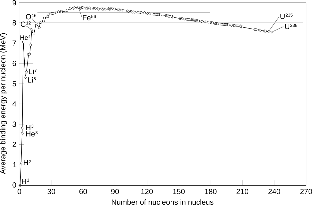
When comparing nuclei with different numbers of nucleons, it is usually more helpful to consider the binding energy per nucleon (\(B/A\)). Figure 12.1 shows the binding energy per nucleon plotted against the mass number \(A\).
Notice the following features:
- For many nuclei: \(\dfrac{B}{A}\approx 8\,\mathrm{MeV}.\)
- The helium-4 nucleus(\(\ele{He}{2}{4}{2}\)) that we know as the \(\alpha\)-particle, is exceptionally tightly bound.
- There is a broad maximum in the iron–nickel region, around \(A\approx60\).
- For \(A\gtrsim20\), the binding energy per nucleon remains roughly constant instead of increasing continuously with \(A\).
This approximate constancy suggests that each nucleon interacts strongly with only a limited number of nearby nucleons. The nuclear interaction is therefore short-ranged and exhibits saturation. - Nuclear processes can release energy when their products lie higher on the binding-energy-per-nucleon curve than their initial nuclei.
- Light nuclei can release energy by combining to form more tightly bound nuclei. This is nuclear fusion.
- Very heavy nuclei can release energy by splitting into more tightly bound medium-mass nuclei. This is nuclear fission.
12.2 Nuclear Decay
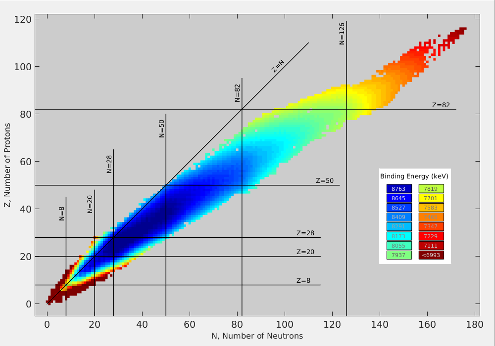

Most known nuclides are unstable and eventually decay into other nuclei. The characteristic timescale of a decay is usually described by the half-life.
Nuclear decay can be thought of as a nucleus moving towards a more energetically favourable configuration. A decay is possible when the final products have a lower total energy than the original nucleus, while also satisfying the relevant conservation laws.
The stable and long-lived nuclei occupy a band on the chart of nuclides commonly called the valley of stability. Figure 12.2 shows the binding energies and half-lives of the known nuclides.
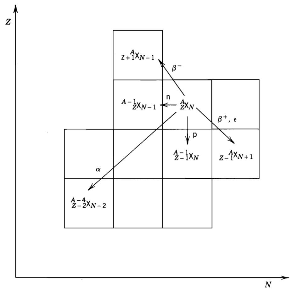
There are several ways in which an unstable nucleus can decay. The most common decay modes are illustrated in Figure 12.3 and summarised in Table 12.3.
| Type of Decay | Generally | Example | Link |
|---|---|---|---|
| \(\alpha\) decay | \(\me{\ele{X}{Z}{A}{N}}{\ele{Y}{Z-2}{A-4}{N-2} + \ele{He}{2}{4}{2}}\) | \(\me{\ele{Ra}{88}{226}{138}}{\ele{Rn}{86}{224}{136} + \alpha}\) | kaeri |
| \(\beta^-\) decay | \(\me{n}{p+e^- + \Aen}\) | \(\me{\ele{C}{6}{14}{8}}{\ele{N}{7}{14}{7}+e^- + \Aen}\) | kaeri |
| \(\beta^+\) decay | \(\me{p}{n+e^+ + \en}\) | \(\me{\ele{Na}{11}{22}{11}}{\ele{Ne}{10}{22}{12}+e^+ + \en}\) | kaeri |
| Electron capture(\(\varepsilon\), EC) | \(\me{p+e^-}{n}\) | \(\me{\ele{Mn}{25}{54}{29}}{\ele{Cr}{24}{54}{30}}\) | kaeri |
| \(\beta\)\(\beta\) decay | \(\me{2n}{2p+2e^+ + 2\en}\) | \(\me{\ele{Ca}{20}{48}{28}}{\ele{Ti}{22}{48}{26}+e^- + \Aen}\) | kaeri |
| \(\gamma\) decay | - De-excitation by the emission of a gamma photon. - When the original state is a meta stable nuclear level (i.e. an isomer) the process is called Internal Transition (IT). |
\(\me{\ele{Co}{27}{60}{33}}{\ele{Co}{27}{60}{33} + \gamma}\) | kaeri |
| Internal Conversion (IC) | Emission of an atomic electron instead of a gamma photon. | \(\me{\ele{Hg}{80}{203}{23}}{\ele{Tl}{81}{203}{24}+e^- + \Aen}\) | kaeri |
| Spontaneous fission | \(^{238}_{92}\mathrm{U}^* \rightarrow ^{140}_{54}\mathrm{Xe}^* + ^{94}_{38}\mathrm{Sr} + 2 ^1_0\mathrm{n} + \gamma\) | kaeri | |
| Nucleon (\(n, p\)) emission | \(\me{\ele{Tm}{69}{147}{}}{\ele{Er}{68}{146}{} + \ele{p}{1}{1}{}}\) | kaeri |
(Note: Similar to internal conversion, atoms can undergo a process called Auger emission, where an electron is ejected instead of an X-ray photon when filling an inner electron vacancy.)
12.2.1 The \(N/Z\) Ratio
For light stable nuclei, particularly those with \(Z\lesssim20\), the numbers of protons and neutrons are approximately equal: \(N\approx Z\) or \(50:50\).
As \(Z\) increases, the electrostatic repulsion between the protons becomes increasingly important. Additional neutrons help to provide more nuclear attraction without adding further electrostatic repulsion. Consequently, the neutron-to-proton ratio of stable nuclei gradually increases.
Typically, \(\dfrac{N}{Z}\approx1.5\) (\(60:40\)) for the heaviest stable nuclei, while the ratio can approach approximately \(\dfrac{N}{Z}\approx1.6\) for very heavy, long-lived nuclei.
12.2.2 Nuclear Magic
The numbers
\[ 2,\ 8,\ 20,\ 28,\ 50,\ 82,\ 126 \tag{12.1}\]
are called magic numbers. Nuclei for which either \(Z\) or \(N\) is a magic number often exhibit enhanced stability. This can appear through properties such as larger nucleon-separation energies and relatively high excitation energies for their first excited states.
A nucleus for which both \(Z\) and \(N\) are magic numbers is called doubly magic.
12.2.3 Being Even Matters
| Z | N | Number of Stable Nuclei |
|---|---|---|
| Even | Even | 165 |
| Even | Odd | 55 |
| Odd | Even | 50 |
| Odd | Odd | 4 |
Table 12.4 summarises the numbers of stable nuclei associated with the different combinations of even and odd \(Z\) and \(N\). As, you can see, it also matters whether a nucleus contains an odd or even number of protons and neutrons. Consequently, even–even nuclei are especially common, whereas stable odd–odd nuclei are rare.
We will see why this is the case when we discuss the Fermi Model.
12.3 Energy Levels, Spin and Parity
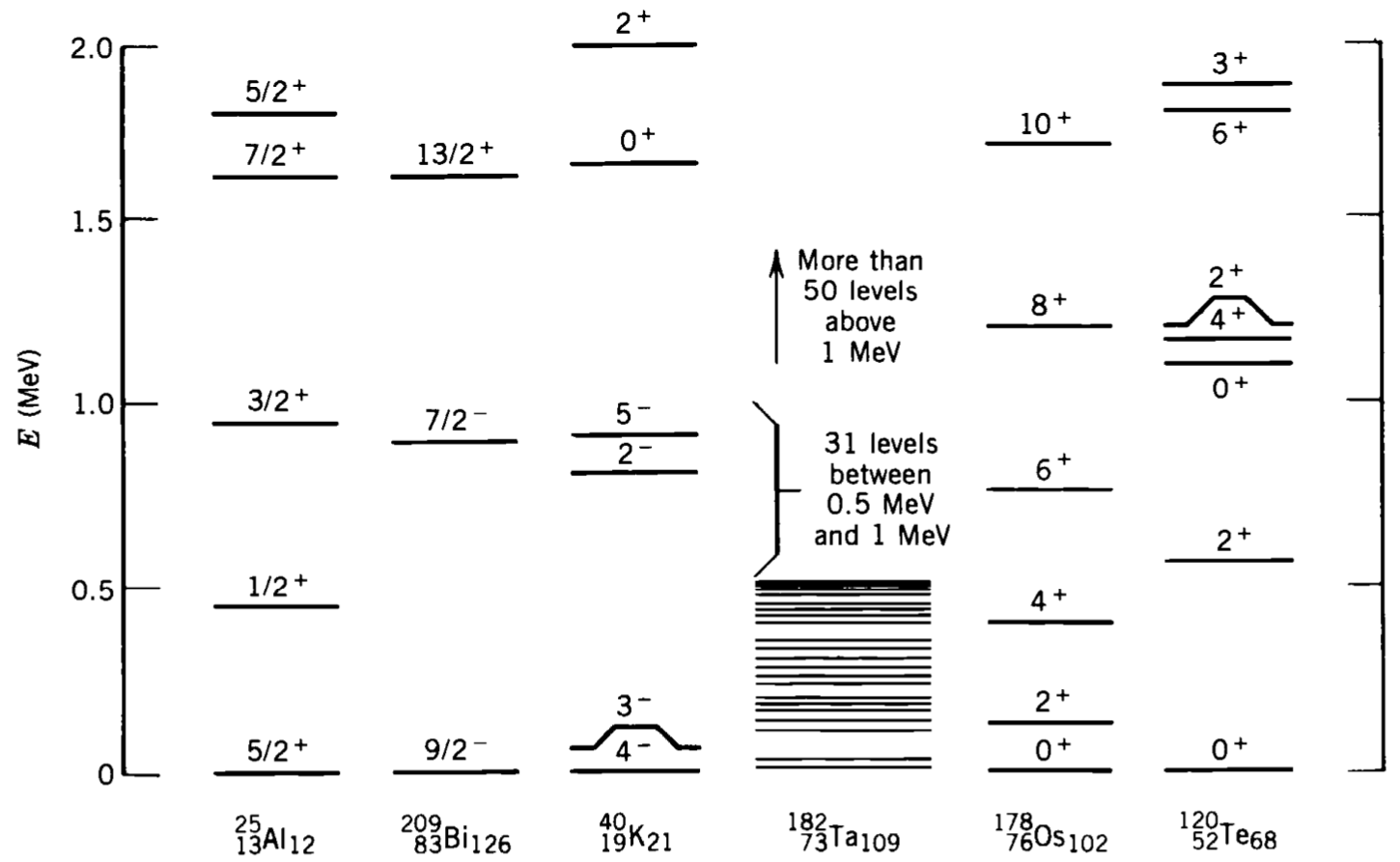
Each nuclear state has a characteristic total angular momentum and parity. The total angular momentum arises from the intrinsic spins and orbital angular momenta of the protons and neutrons. Parity describes how the nuclear wavefunction behaves under spatial inversion. It is common to express these two properties together as \(J^\eta\).
A nucleus can exist in different excited states, much like an atom. These excited states are generally unstable and eventually decay towards the ground state, which is the lowest-energy state of the nucleus. Some excited states can nevertheless be relatively long-lived and are known as metastable states or nuclear isomers.
Figure 12.5 shows some of the excited energy levels of several nuclei. Notice that nuclear energy-level separations are commonly in the \(\mathrm{keV}\) to \(\mathrm{MeV}\) range, compared with the \(\mathrm{eV}\) scale typical of atomic-electron excitations.
Different nuclear states can also have different properties, including their size, shape, spin, parity, magnetic dipole moment and electric quadrupole moment. In this chapter (and for much of this course) we will focus mainly on the properties of nuclei in their ground states.
12.4 Size of the Nucleus
12.4.1 Not a Point, Not a Sphere
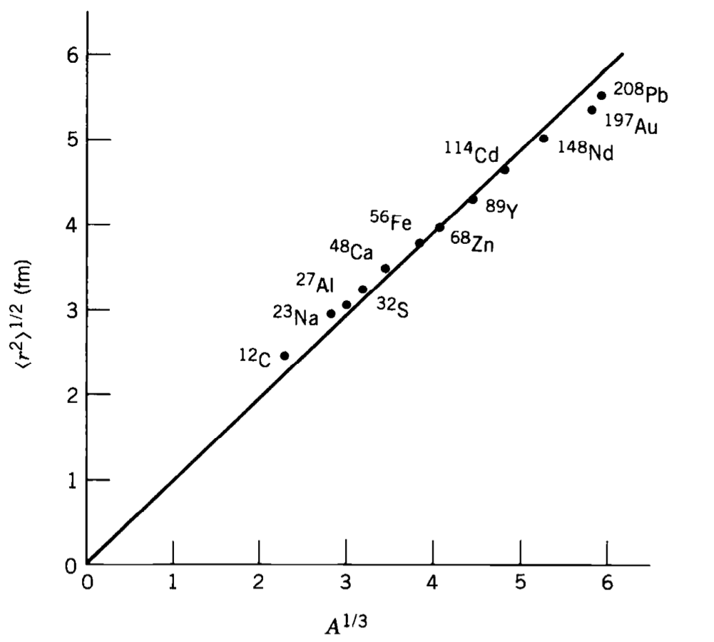
To begin, the nucleus is not a point, nor is it generally spherical. Nevertheless, it is convenient to define a characteristic radius that allows us to compare different nuclei.
A useful quantity is the mean-square charge radius, defined as
\[ \langle r^2\rangle = \frac{ \displaystyle\int_{\text{all space}} r^2\rho(\v{r})\,d^3r }{ \displaystyle\int_{\text{all space}} \rho(\v{r})\,d^3r }, \tag{12.2}\]
where \(\rho(\v{r})\) is the nuclear charge density.
The corresponding root-mean-square charge radius is
\[ r_{\mathrm{rms}} = \sqrt{\langle r^2\rangle}. \tag{12.3}\]
If you are wondering why \(\langle r^2\rangle\) is preferred over \(\langle r\rangle\), it is because the former is more directly related to many experimental measurements.
It has been experimentally established that the number of nucleons per unit volume is roughly constant across most nuclei. If we approximate the nucleus as a sphere, then
\[ \frac{A}{\frac{4}{3}\pi R^3} \approx \text{constant}. \tag{12.4}\]
This leads to the useful empirical radius formula
\[ { R=R_0A^{1/3} }, \tag{12.5}\]
where
\[ R_0\approx1.2\,\mathrm{fm}. \]
The measurements in Figure 12.6 support the characteristic \(A^{1/3}\) dependence. Note, however, that the quantity plotted on the vertical axis is \(r_{\mathrm{rms}}=\sqrt{\langle r^2\rangle}\), whereas the \(R\) appearing in Equation 12.5 is an effective nuclear radius.
For a uniform spherical charge distribution, these quantities are related by
\[ r_{\mathrm{rms}} = \sqrt{\frac{3}{5}}\,R. \tag{12.6}\]
Thus, the coefficient obtained by fitting RMS radii is smaller than the commonly quoted value \(R_0\approx1.2\,\mathrm{fm}\).
12.4.2 Charge and Matter Distributions
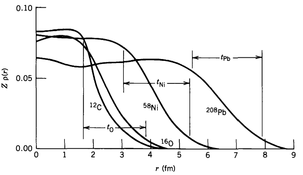
Let us now discuss how charge and matter are distributed inside the nucleus.
One of the most direct ways to probe the nuclear interior is to scatter high-energy electrons from nuclei. Electrons are particularly useful because they do not participate in the strong interaction. Their scattering therefore primarily probes the nuclear charge distribution through the electromagnetic interaction.
Figure 12.7 shows charge distributions extracted from elastic electron-scattering measurements.
Notice that:
- the central charge density varies somewhat between nuclei;
- heavier nuclei have larger characteristic radii, as described by Equation 12.5;
- the charge density is approximately constant through much of the nuclear interior;
- all the distributions have similar diffuse edge profiles.
A useful representation of the nuclear charge distribution is the Woods–Saxon distribution:
\[ \rho(r) = \f{\rho_0}{1 + \text{exp}\lr{\f{r-R}{a}}} \tag{12.7}\]
The parameters are summarised below:
| \(\rho_0\) | Is a constant that gives the correct charge via \(\displaystyle\int \rho(r)d^3 r = Z\) |
| \(R\) | Mean Nulcear Radius, where the density drops to \(\frac{1}{2}\) of the central density. |
| \(a\) | Is a constant that determines the width of the changing edge region. or many medium and heavy nuclei, \(a\approx0.5\,\mathrm{fm}.\) |
The ‘diffuseness’ of the nuclear surface can also be described using the skin thickness, \(t\). This is the distance over which the density falls from 90% to 10% of its central value.
For the Woods–Saxon distribution, \[ t=4a\ln3. \tag{12.8}\]
With \(a\approx0.5\,\mathrm{fm}\), this gives
\[ t\approx2.2\,\mathrm{fm}. \]
Since the nucleus contains both protons and neutrons, we might ask whether the distribution of matter (the matter radius) is the same as the distribution of charge (the charge radius).
For many stable nuclei, the charge and matter radii are quite similar, and both approximately follow the \(A^{1/3}\) dependence of Equation 12.5. However, significant differences can occur in nuclei far from stability.
12.4.3 Scattering Experiments for Size
We can use scattering experiments to probe nuclear charge and matter distributions. Electrons primarily probe the charge distribution, while strongly interacting particles such as protons, neutrons and \(\alpha\)-particles can provide information about the matter distribution.
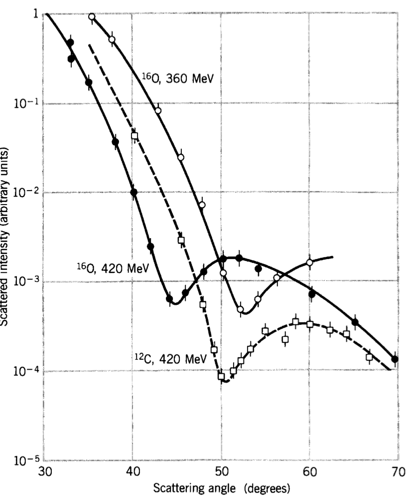
Figure 12.8 shows elastic electron-scattering measurements performed using electrons with energies of approximately 360 and 420 MeV incident on carbon and oxygen nuclei.
The measured angular distributions contain distinctive patterns resembling the diffraction patterns produced by light waves. This is not a coincidence: both phenomena involve waves scattering from objects with finite spatial dimensions.
For light diffracted by a circular aperture or disk of diameter \(D\), the first minimum occurs approximately at
\[ \sin\theta_{\min} = \frac{1.22\lambda}{D} \qquad\Rightarrow\qquad \theta_{\min} = \sin^{-1}\left(\frac{1.22\lambda}{D}\right). \tag{12.9}\]
This optical analogy allows us to obtain a rough estimate of the size of the nuclear charge distribution from the positions of the diffraction minima.
However, a nucleus is three-dimensional, and its charge distribution does not have a perfectly sharp edge. Consequently, the positions and depths of the minima differ from those predicted by the simple two-dimensional disk model.
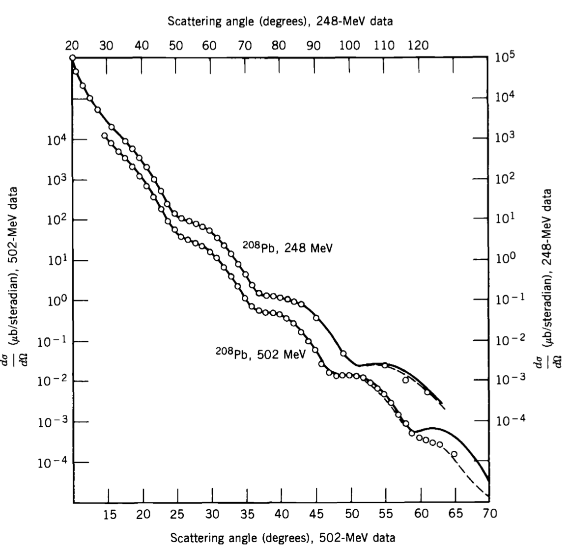
As illustrated in Figure 12.9, a more sophisticated treatment is required to extract quantitative information about the charge distribution. Let me sketch the basic idea.
12.4.4 Form Factors
Consider electrons that are elastically scattered from a nuclear charge distribution \(\rho(\v{r})\). Let the initial and final electron momenta be
\[ \v{p}_i=\hbar\v{k}_i \qquad\text{and}\qquad \v{p}_f=\hbar\v{k}_f. \tag{12.10}\]
The corresponding plane-wave states may be written as
\[ \begin{aligned} \psi_i(\v{r},t) &= \frac{1}{\sqrt{L^3}} e^{i(\v{k}_i\cdot\v{r}-\omega_i t)}, \\ \psi_f(\v{r},t) &= \frac{1}{\sqrt{L^3}} e^{i(\v{k}_f\cdot\v{r}-\omega_f t)}, \end{aligned} \tag{12.11}\]
Where, I have placed my experiment in a huge cubic box of size \(L\) for the sake of normalisation. \(L\) will eventually disappear, so do not worry about it.
The probability of scattering is related to the matrix element of the interaction potential:
\[ \mathcal M_{fi} = \langle\psi_f|V(\v r)|\psi_i\rangle. \tag{12.12}\]
Here, \(V(\v r)\) is the potential energy of the electron due to the nuclear charge distribution \(\rho(\v r)\).
The matrix element is a scattering amplitude. The probability, and hence the cross-section, depends on its modulus squared:
\[ P_{i\rightarrow f} \propto |\mathcal M_{fi}|^2. \tag{12.13}\]
Let us explore the matrix element a little further. Written as an integral,
\[ \begin{align} \mathcal M_{fi} &= \langle\psi_f|V(\v r)|\psi_i\rangle \\ &= \int \psi_f^*(\v r)\, V(\v r)\, \psi_i(\v r)\, \dd[3]{r} \\ &= \frac{1}{L^3} \int e^{-i\v q\cdot\v r/\hbar} V(\v r)\, \dd[3]{r}. \end{align} \tag{12.14}\]
Here, for convenience, I have introduced the momentum-transfer vector
\[ \v q = \v p_f-\v p_i = \hbar(\v k_f-\v k_i). \tag{12.15}\]
Let us pause here to note that Equation 12.14 tells us that the scattering amplitude is related to the Fourier transform of the scattering potential.
The specific information about the nuclear charge distribution is contained in \(V(\v r)\) through:
\[ V(\v r) = -\frac{e}{4\pi\epsilon_0} \int \frac{\rho(\v r')} {\lra{\v r-\v r'}} \,\dd[3]{r'}. \tag{12.16}\]
Here, \(\rho(\v r)\) is the nuclear charge density, normalised so that
\[ \int \rho(\v r)\, \dd[3]{r} = Ze. \tag{12.17}\]
Combining the Fourier-transform relation for the scattering amplitude with the Coulomb potential leads to the quantity
\[ { F(\v q) = \frac{1}{Ze} \int \rho(\v r) e^{-i\v q\cdot\v r/\hbar} \,\dd[3]{r} }. \tag{12.18}\]
\(F(\v q)\) is called the nuclear scattering form factor. It contains information about the spatial distribution of nuclear charge.
The form factor is essentially the Fourier transform of the nuclear charge distribution. Different values of momentum transfer probe different spatial scales within the nucleus.
Note that, for zero momentum transfer,
\[ F(\v 0) = \frac{1}{Ze} \int \rho(\v r)\, \dd[3]{r} = 1. \tag{12.19}\]
If the charge distribution is spherically symmetric, the form factor simplifies to
\[ { F(q) = \frac{4\pi}{Ze} \int_0^\infty \rho(r) \frac{\sin(qr/\hbar)}{qr/\hbar} r^2\,dr }. \tag{12.20}\]
In the plane-wave Born approximation, the finite-size and point-nucleus differential cross-sections are related by:
\[ { \left(\frac{d\sigma}{d\Omega}\right)_{\mathrm{finite\ size}} = \left(\frac{d\sigma}{d\Omega}\right)_{\mathrm{point}} |F(q)|^2 }. \tag{12.21}\]
By fitting measurements such as those shown in Figure 12.8 and Figure 12.9 using Equation 12.21, we can infer the nuclear charge distribution.
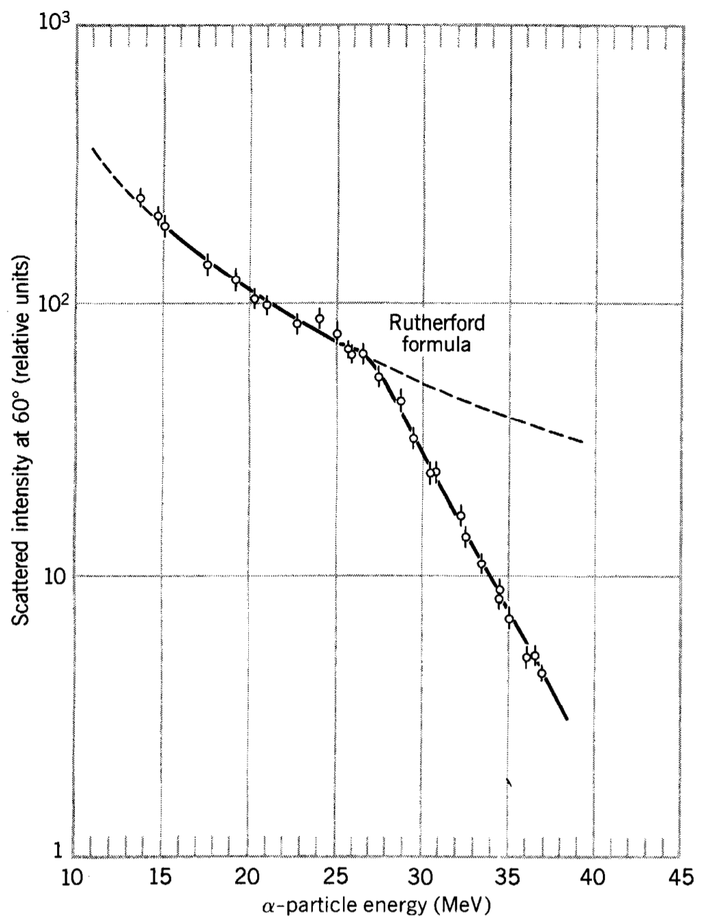
If we want to probe the matter distribution, we need a projectile that interacts through the strong nuclear force. Neutrons, protons and ions such as \(\alpha\)-particles can be used for this purpose.
The interpretation is more complicated because charged projectiles experience both the Coulomb and strong interactions. At sufficiently low energies, the projectile remains mostly outside the nucleus, and its scattering may be described primarily by the Coulomb interaction. As its energy increases and it approaches the nuclear surface more closely, the strong interaction begins to influence the scattering.
The resulting departure from Rutherford scattering, illustrated in Figure 12.10, provides information about the nuclear matter distribution and the nuclear interaction.
12.5 Shape of the Nucleus
12.5.1 Electric Moments
Let us now focus on the shape of the nucleus. Since nuclei are extremely small, ordinary microscopy is not possible. However, we can obtain information about the distribution of nuclear charge, and hence about nuclear shape, by studying electric moments.
The various electric multipoles carry different information about the original charge distribution.
\[ \def\r{\v{r}} \def\rp{\v{r'}} \newcommand\x[1]{\small\displaystyle\int \rho(\rp) {#1}\,d^3r'} \]
| Moment | Expression | What it tells us |
|---|---|---|
| \(E0\) (monopole) |
\(\x{}=Ze\) | The total nuclear charge, \(Ze\). |
| \(E1\) (dipole, \(p\)) |
\(\x{r'\cos\theta}=\x{z'}\) | A separation of positive and negative charge. |
| \(E2\) (quadrupole, \(Q\)) |
\(\x{\frac{1}{2}r'^2(3\cos^2\theta-1)}=\x{\frac{1}{2}(3z'^2-r'^2)}\) | Whether the charge distribution is stretched along, or spread away from, a chosen direction. |
The electric monopole moment gives only the total nuclear charge and conveys no information about shape. For a stationary nuclear state with definite parity, the permanent electric dipole moment is zero. The next electric moment that can reveal information about nuclear shape is therefore the electric quadrupole moment.
Higher electric moments, such as octupole moments, can describe more complicated charge distributions. We will focus mainly on the quadrupole moment, which gives the simplest useful measure of nuclear deformation.
For an axially symmetric charge distribution, it is usual to define the intrinsic quadrupole moment as
\[ Q_0 = \frac{1}{e} \int \rho(\v r') \left(3z'^2-r'^2\right) \dd[3]{r'}. \tag{12.22}\]
Here, \(\rho(\v r')\) is the nuclear charge density and \(z'\) is the intrinsic symmetry axis of the nucleus. The factor \(1/e\) means that \(Q_0\) has units of area. Nuclear quadrupole moments are therefore usually quoted in barns (\(1\,\mathrm{b}=10^{-28}\,\mathrm{m^2}\)).
12.5.2 Shape from Electric Moments
The quadrupole moment compares the amount of charge distributed along the intrinsic symmetry axis with the amount distributed perpendicular to it.
| Shape | Quadrupole moment | Interpretation |
|---|---|---|
| Prolate spheroid (cigar-like in \(z'\)) |
\(Q_0>0\) | More charge is distributed along the \(z'\)-axis. |
| Spherical distribution | \(Q_0=0\) | The charge distribution is the same in every direction. |
| Oblate spheroid (squashed in \(z'\)) |
\(Q_0<0\) | More charge is distributed perpendicular to the \(z'\)-axis. |
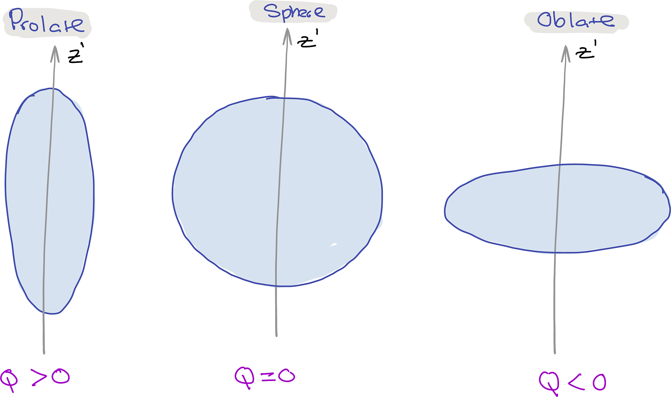
Thus, a non-zero intrinsic quadrupole moment indicates that the nuclear charge distribution is not spherical. However, a measured quadrupole moment of zero does not always prove that a nucleus is intrinsically spherical. The reason for this is interesting and subtle. The quadrupole moment defined in Equation 12.22 refers to the nucleus in its own body-fixed frame. Experiments measure a related laboratory-frame quantity called the spectroscopic quadrupole moment, \(Q_s\).
To measure \(Q_s\), we first need a laboratory direction with which to compare the nuclear charge distribution. An external magnetic field commonly supplies this direction by defining the axis along which the nuclear angular momentum is described.
- If \(J=0\), the laboratory state has no preferred direction. Thus, even if \(Q_0\neq0\), the measured spectroscopic quadrupole moment is \(Q_s=0\).
- If \(J=\tfrac12\), the possible alignments are still ‘insufficient’ to give a measurable quadrupole moment, so \(Q_s=0\) (see problem set to figure out why).
- A non-zero \(Q_s\) can be measured only for nuclei with \(J\geq1\).
12.6 Magnetic Dipole Moment
The magnetic dipole moment of a nucleus is another important parameter. It tells us how the nucleus responds to an external magnetic field and therefore can provides information about the angular momenta of its constituent nucleons. Nuclear magnetic moments can be probed through experiments such as nuclear magnetic resonance (NMR), hyperfine spectroscopy, and nuclear-spin alignment.
We saw in the previous chapter how the orbital magnetic dipole moment is related to angular momentum:
\[ \v{\mu}=\frac{q}{2m}\v{L}. \tag{12.23}\]
The quantum-mechanical is:
\[ \hat{\v\mu}_{\mathrm{orb}} = \frac{q}{2m}\hat{\v L}. \tag{12.24}\]
In experiments involving an external magnetic field, it is natural to choose the \(z\)-axis to lie along the field direction. The angular-momentum component along this direction then has definite allowed values:
\[ \hat L_z\ket{\ell,m_\ell} = m_\ell\hbar\ket{\ell,m_\ell}. \]
Here, \(m_\ell=-\ell,-\ell+1,\ldots,\ell\) labels the allowed orientations of the orbital angular momentum relative to the magnetic field.
Therefore, the corresponding orbital magnetic-moment component is
\[ \mu_z = \frac{q\hbar}{2m}m_\ell. \tag{12.25}\]
The possible values of the magnetic moment are therefore linked directly to the allowed values of \(m_\ell\).
12.6.1 Measuring \(\boldsymbol \mu\)
We can know \(L^2\) and one component of angular momentum simultaneously (here we have chosen \(L_z\)). The state has rotational symmetry about the \(z\)-axis, so there is no preferred direction in the \(x\)–\(y\) plane. So, for a state of definite \(\ell\) and \(m_\ell\), the transverse components of the angular momentum have zero expectation value:
\[ \langle L_x\rangle=\langle L_y\rangle=0, \qquad \langle L_z\rangle=m_\ell\hbar. \]
In a semiclassical picture, \(\v L\) precesses about the \(z\)-axis, and its transverse components average to zero. Hence, for such a case:
\[ \langle\v\mu_{\mathrm{orb}}\rangle = \frac{q}{2m}\langle\v L\rangle = \frac{q}{2m}m_\ell\hbar\,\hat{\v z}. \]
12.6.2 Magnetons
Two convenient units for expressing magnetic dipole moments are:
| Definition | Value | |
|---|---|---|
| Nuclear magneton | \(\mu_\text{N}=\dfrac{e\hbar}{2m_p}\) | \(3.15245\times10^{-8}\,\mathrm{eV/T}\) |
| Bohr magneton | \(\mu_\text{B}=\dfrac{e\hbar}{2m_e}\) | \(5.78838\times10^{-5}\,\mathrm{eV/T}\) |
Since \(\mu_\text{B}\gg\mu_\text{N}\), electronic magnetic moments are much larger than nuclear magnetic moments. Nevertheless, nuclear magnetic moments are measurable and are responsible for effects such as the hyperfine splitting of atomic spectral lines.
12.6.3 Including Spin
A particle’s intrinsic spin angular momentum also contributes to its magnetic dipole moment.
For a nucleon, we write
\[ \v\mu = \mu_\text{N} \left( g_\ell\frac{\v L}{\hbar} + g_s\frac{\v S}{\hbar} \right), \tag{12.26}\]
| Nucleon | \(g_\ell\) | \(g_s\) |
|---|---|---|
| Proton | \(1\) | \(5.586\) |
| Neutron | \(0\) | \(-3.826\) |
where \(g_\ell\) and \(g_s\) are called \(g\) factors. They specify how strongly the orbital angular momentum and intrinsic spin angular momentum contribute to the magnetic moment.
The commonly used free-nucleon values are shown in the table.
You can make sense of \(g_{l,p}=1\) and \(g_{l,n}=0\) by recalling the simple picture of a current loop. The proton has an orbital magnetic contribution because it is charged: its orbital motion constitutes a current. The neutron has no orbital contribution in this simple picture because it has no net charge.
However, although the neutron has no net electric charge, it still has an intrinsic spin magnetic moment. This is an important observation: it indicates that the neutron has internal structure, which we now understand in terms of its charged quark constituents.
For a nucleus, we add the contributions from all its nucleons:
\[ { \v\mu_{\mathrm{nucleus}} = \mu_\text{N} \sum_i \left( g_{\ell,i}\frac{\v L_i}{\hbar} + g_{s,i}\frac{\v S_i}{\hbar} \right) }. \tag{12.27}\]
The sum includes orbital motion of the protons and intrinsic-spin contributions from both protons and neutrons.