10 Particle Interactions: Processes

What To Expect In This Chapter

The previous chapter focused on the probability that an interaction between radiation and matter will occur. That discussion was quite general and applied to many different forms of radiation.

We now turn to what happens during an interaction. The mechanisms available depend on the type of radiation involved, for example, whether it is charged or uncharged, light or heavy, and fast or slow.

10.1 Heavy Charged Particles

10.1.1 Kinematics

Let us begin by considering how a heavy charged particle, by which I mean a particle much heavier than an electron, propagates through matter.

A heavy charged particle can interact with both the nuclei and the atomic electrons in the material. Scattering from nuclei can be described, approximately, using the Rutherford cross-section. However, energy loss through interactions with atomic electrons is usually much more frequent and is the dominant mechanism over a broad range of projectile energies.

The electrons occupy a much larger region of the atom than the nucleus, so an incoming charged particle encounters their electric fields frequently. However, the large mass difference between the heavy projectile and an electron means that only a small fraction of the projectile’s energy can be transferred in any single collision.

We can get a feel for this by considering a non-relativistic elastic collision; Equation 10.1 gives the energy transferred to an initially stationary electron as

\[ \begin{aligned} T &= E_0 \frac{4m_eM}{(m_e+M)^2} \sin^2\left(\frac{\theta^*}{2}\right) \\ &= E_0 \frac{4m_e/M}{(m_e/M+1)^2} \sin^2\left(\frac{\theta^*}{2}\right). \end{aligned} \]

Since

\[ M\gg m_e, \]

we have

\[ { T \approx \frac{4m_e}{M} E_0 \sin^2\left(\frac{\theta^*}{2}\right) }. \tag{10.1}\]

Here, \(M\) and \(E_0\) are the mass and initial kinetic energy of the heavy projectile, while \(\theta^*\) is the projectile’s scattering angle in the CM frame.

The maximum energy transfer occurs when \(\theta^*=\pi,\) and is therefore \[ { T_{\max} \approx \frac{4m_e}{M}E_0 }. \]

Because \(m_e/M\) is very small, even the maximum possible energy transfer is only a small fraction of the projectile’s initial energy. A heavy charged particle must therefore undergo many interactions before losing a substantial amount of energy.

We can also use Equation 8.25 to examine the direction of the projectile after a collision. For a heavy projectile of mass \(M\) colliding with an electron of mass \(m_e\),

\[ \zeta=\frac{M}{m_e}\gg1. \]

Therefore,

\[ \tan\theta = \frac{\sin\theta^*} {\cos\theta^*+\zeta} \approx \frac{m_e}{M}\sin\theta^*. \]

Hence,

\[ \theta\approx0. \]

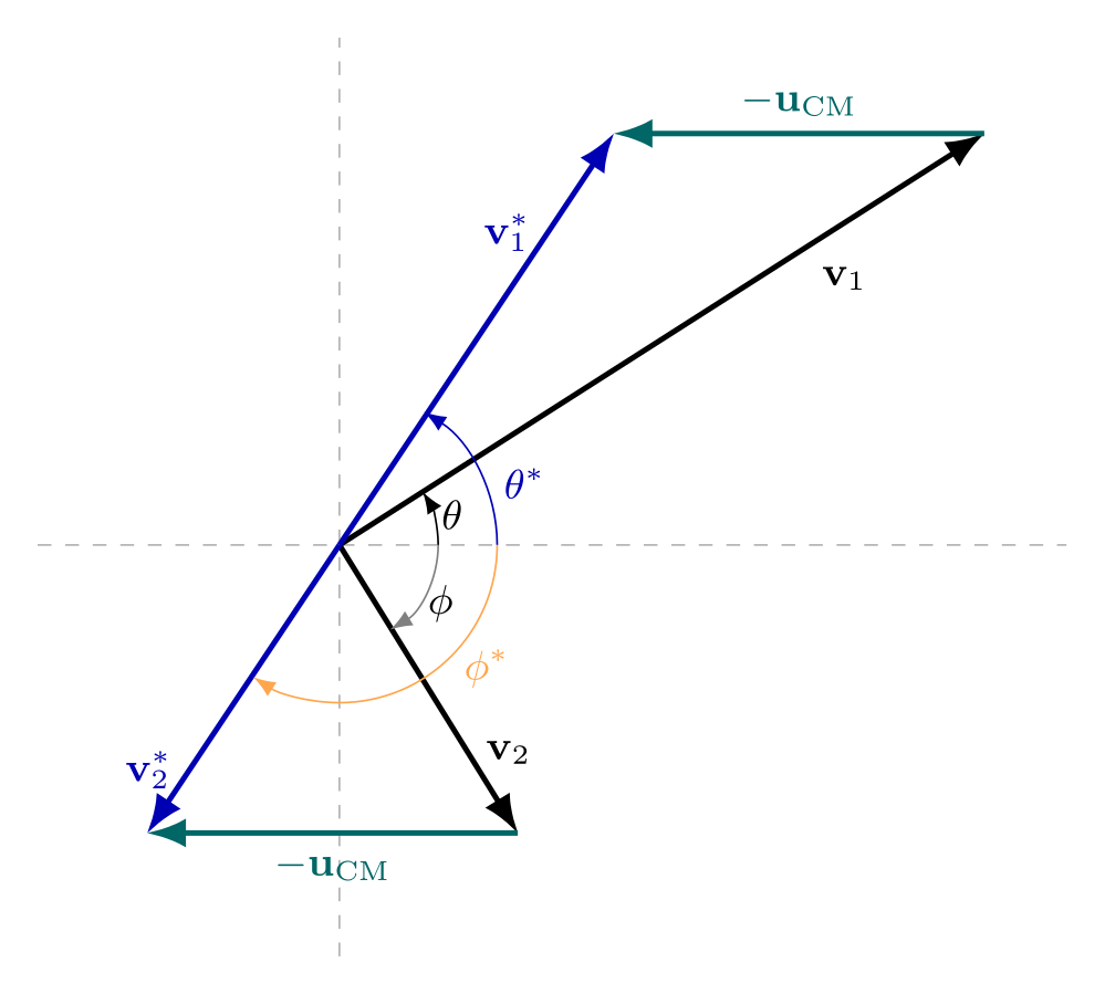
Figure 10.1: Relationship between the various velocities in the LAB and CM frames after a two-body collision.

Thus, each collision produces only a very small change in the direction of the heavy projectile. Its trajectory through the material is therefore approximately straight, even though it undergoes many interactions along the way.

As seen in Figure 10.1 the recoil angle \(\phi\) of the electron in the LAB frame is related to the CM scattering angle by

\[ \theta^*=\pi-2\phi \Rightarrow \phi=\frac{\pi}{2}-\frac{\theta^*}{2}. \]

For collisions with small \(\theta^*\),

\[ \phi\approx\frac{\pi}{2}. \]

In such collisions, the recoil electron moves approximately perpendicular to the original direction of the heavy projectile. Consequently, some of the energy deposited by the projectile spreads laterally away from its primary path. These electrons are sometimes called \(\delta\)-rays and erode the resolution of ion beam lithographic processes.

10.1.2 Bethe Model For Energy Loss

Ions participate in many, many ion-electron collisions. So, although the energy transferred is small, the sheer number of collisions makes electron interactions the primary mode of energy loss for ions. In 1930, Hans Bethe formulated a theoretical relationship for this energy loss that goes like this:

\[ \dfrac{dE}{dx}=\left(\dfrac{e^{2}}{4 \pi \epsilon _{0}}\right) ^{2} \dfrac{4 \pi z^{2}N _{A}Z\rho }{m_e c^{2}\beta ^{2}A} \left[ \ln \left( \dfrac{2m_e c^{2}\beta ^{2}}{I}\right) -\ln \left( 1-\beta ^{2}\right) -\beta ^{2}\right] \tag{10.2}\]

Where,

\(Z\)	Atomic number of the target material
\(z\)	Charge of the projectile
\(\beta = v/c\)	where \(v\) is the speed of the projectile
\(A\)	Atomic mass of the target material
\(\rho\)	Density of the material
\(N_A\)	Avogardro constant

The parameter \(I\) is the mean excitation energy of the atomic electrons. We can refer to experimental data for values of \(I\) (for instance here from NIST), although several approximations (e.g. \(I = (22.8 + 9.7\text{eV})\cdot Z\,\)) can also be used.

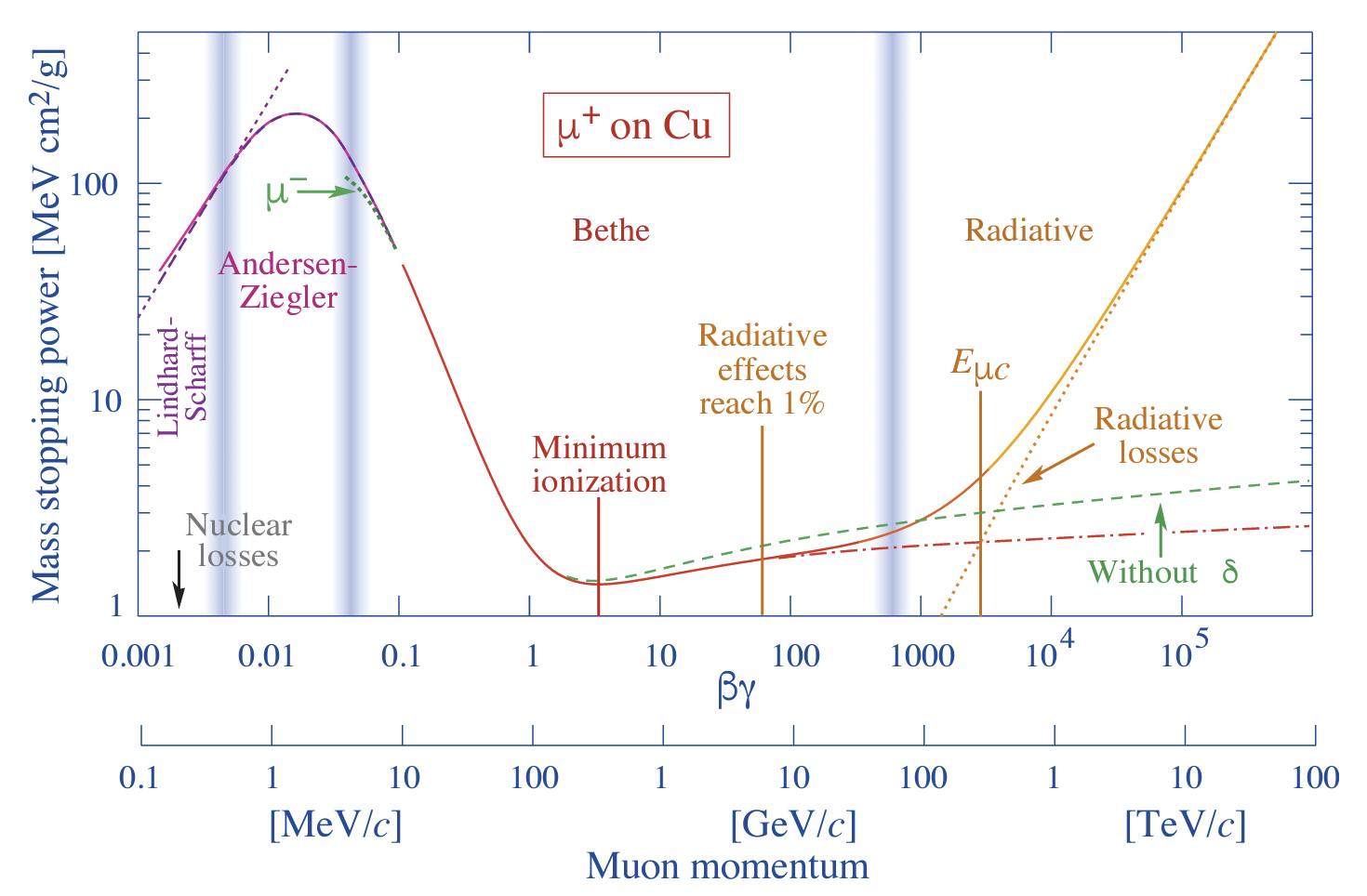
Relationship 10.2 is not perfect and fails at low energies primarily because it does not account for electron capture by the ion. It also fails at higher energies due to radiation effects. You can get a better idea of this by looking at the following figure from The Review of Particle Physics by (¹). It shows the mass stopping power (\(dE/\rho dx\)) for positive muons in copper as a function of \(\beta\gamma = (p/Mc)\) over nine orders of magnitude in momentum (12 orders of magnitude in kinetic energy). Solid curves indicate the total stopping power. The vertical bands indicate boundaries between different approximations, such as the Bethe formula.

Figure 10.2: Bethe stopping-power regimes

10.1.3 Stopping Power

You often see the term stopping power to describe energy loss. The stopping power can be either the linear stopping power(e.g. in MeV/cm) or the mass stopping power(e.g. in MeV cm\(^2\)/g). The linear stopping power is energy lost per unit length while the mass stopping power is energy lost per unit length divided by the density. It can be confusing to figure out which is which; just remember that the one with the units per mass (e.g. MeV cm\(^2\)/g) is the ‘mass’ version.

\[ \lr{\da{E}{x}}_\text{mass}=\f{1}{\rho}\lr{\da{E}{x}}_\text{linear} \tag{10.3}\]

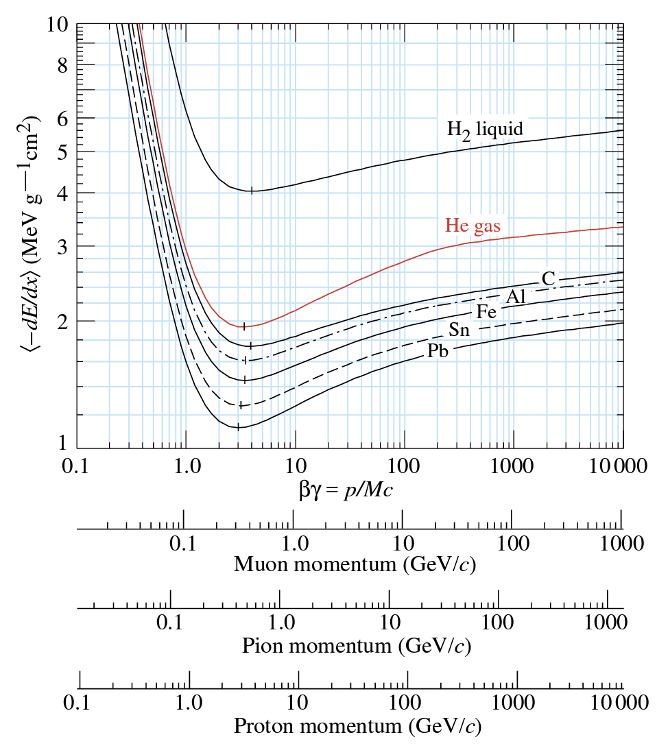
Mass stopping power defined in this way is about the same for most materials, decreasing slowly with \(Z\) as seen in the plot below.

Figure 10.3: Mass stopping power by material

10.1.4 Range Of Ions

We can use the stopping power to determine the range of a particle as follows:

\[ \begin{align} dE &= - \lr{\da{E}{x}}dx \\ \Rightarrow \f{dE}{-dE/dx} &= dx \\ \Rightarrow \int_E^0 -\f{dE}{dE/dx} &= \int_{0}^R dx\\ R &= \int_E^0 \lr{-\da{E}{x}}^{-1}dE\\ \end{align} \]

There is also a semi-empirical relationship called the Bragg-Kleeman rule that allows us to estimate the range of an unknown material from a known one. It goes like this:

\[ \dfrac{\rho _{?}R_{?}}{\rho R}=\sqrt{\dfrac{A_{?}}{A}} \tag{10.4}\]

Where I have used \(?\) to indicate the material whose range is unknown.

10.1.5 Bragg’s Peak

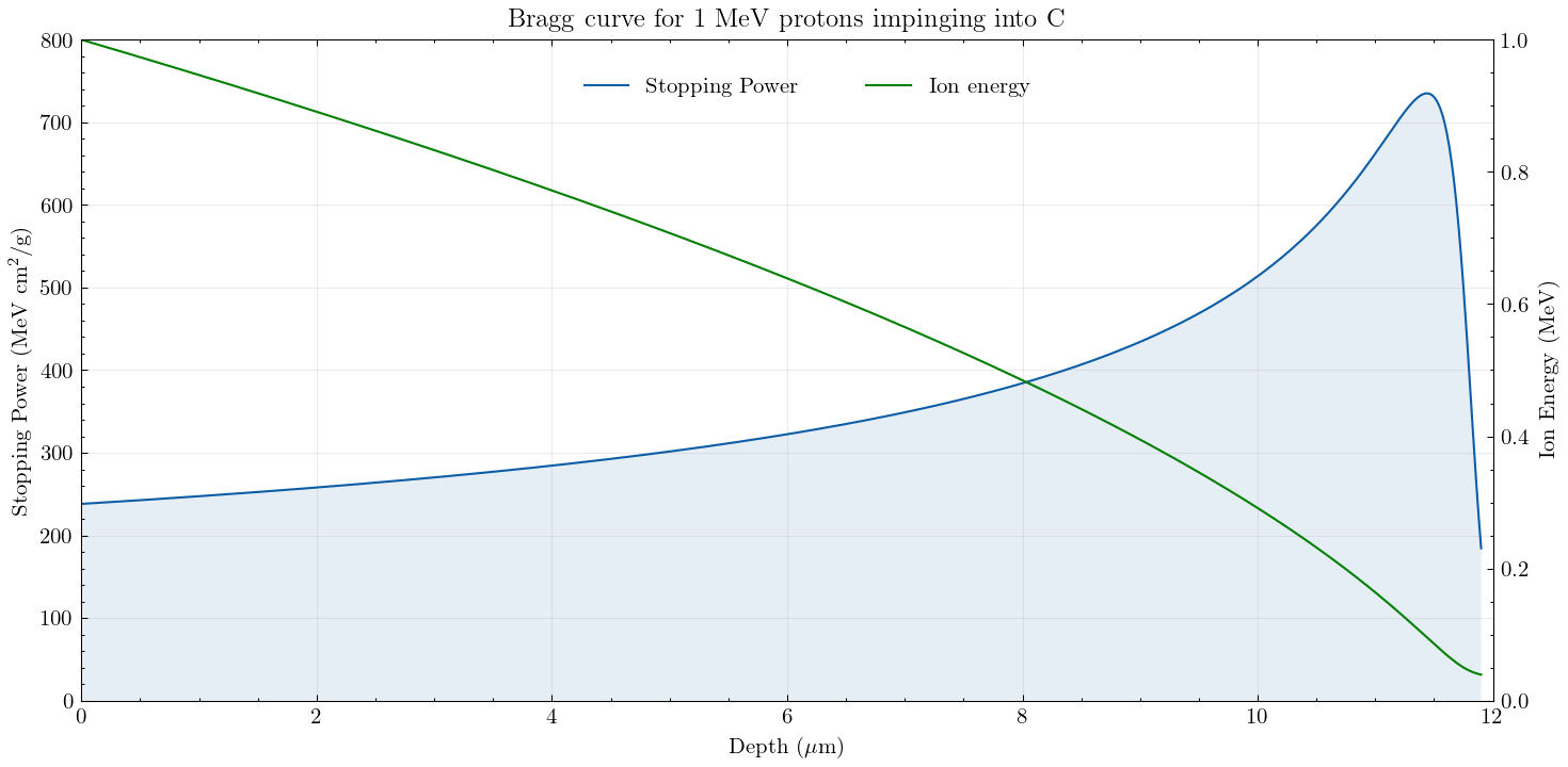
If you look at the Bethe equation (Equation 10.2), you will notice \(1/c^2\beta^2 = v^2\) in the denominator. This results in the stopping power increasing as an ion slows down. This slowing down leads to an important phenomenon called the Bragg peak. You can see it in the figure below, where I have plotted the stopping power with the depth penetrated by the ion. This phenomenon is important because we can tweak the initial energy of the ion so that it stops at a specific depth. This is the basis of proton therapy, where ions can be used for precision damage to cells (e.g. a tumour) at a particular depth.

10.1.6 The Continuous Slowing Down Approximation (Csda)

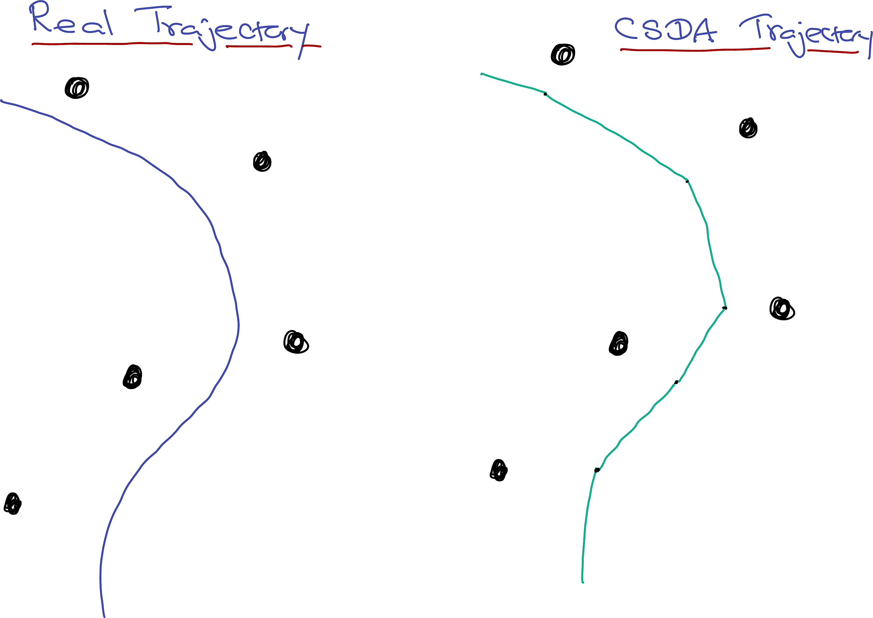
Figure 10.5: Meaning of Continuous Slowing Down Approximation

The picture we have so far is that an ion loses most of its energy through collisions with electrons, but these collisions have little effect on the direction of propagation. The direction is changed significantly by Rutherford-like collisions with the nuclei, which also cause some energy loss. The most significant source of energy loss, however, is still the electrons. It is, therefore, tempting to visualise (and model) the ion’s journey through matter as a sequence of straight-line sprints between nuclear scattering events. The ion loses energy continuously during these inter-nuclear sprints. This is called the Continuous Slowing Down Approximation (CSDA). The distance between nuclear interactions is Poisson distributed according to equation Equation 9.45. This, in turn, will ensure that we end up with the correct mean-free path of equation Equation 9.46. CSDA is a simple model often used in simple Monte-Carlo simulations such as CASINO and SRIM (srim.org).

10.2 Electrons

Now let’s look at how electrons move through matter. Electrons, like heavy ions, also interact with nuclei and suffer changes in direction. They also interact with other electrons and lose energy. However, because the projectiles (electrons) in this case have the same mass, their trajectories are erratic and tortuous. This ultimately leads to a pear-shaped ionisation volume, making it challenging to define a range for electrons that depends on its path. Instead, we use the linear range of the pear-shaped value, as seen in the above image. A quick look at the equation Equation 10.1 indicates that the projectile can transfer all of its energy in a head-on collision. Since there are large exchanges of energy, it becomes difficult to distinguish between the projectile and target electrons. Furthermore, the typical electron energies in nuclear reactions are of the order of MeV, making it necessary to always use relativistic calculations.

Further, the many scattering events that lead to the erratic paths of the electrons mean that they are subject to large accelerations. Since accelerating charges radiate energy, electrons lose a lot of their energy as radiation. This radiation is called bremsstrahlung (German for ‘braking radiation’).

10.2.1 Energy Loss

In addition to the electron-electron scattering, we must incorporate bremsstrahlung into the energy loss of electrons. In the following the subscripts \(c\) and \(r\) stand for the energy loss due to collision and radiation respectively. \(T\) is the electron’s kinetic energy, and the rest of the symbols are similar to that for heavy charged particles. The equation for radiative loss is only valid at relativistic energies. Below \(\approx 1\)MeV, the radiation losses are negligible. \[ \da{E}{x}= \lr{\da{E}{x}}_c+\lr{\da{E}{x}}_r \tag{10.5}\]

Figure 10.7: Electron collisional and radiative losses

\[ \begin{aligned} \lr{\dfrac{dE}{dx}}_c=\left(\dfrac{e^{2}}{4\pi \epsilon _{0}}\right)^{2}\dfrac{2 \pi z^{2}N _{A}Z\rho }{m_e c^{2}\beta ^{2}A}& \left\{\ln\left[\dfrac{T(T + m_e c^{2})^2\beta^{2}}{2I^2 m_e c^2}\right]\right. \\ &\qquad+\lr{1-\beta^{2}}\\ &\qquad-\lr{2\sqrt{1-\beta^{2}}-1+\beta^2}\ln 2 \\ &\qquad\left.+ \frac{1}{8}\lr{1-\sqrt{1-\beta^{2}}}^2\right\} \end{aligned} \tag{10.6}\] \[ \lr{\dfrac{dE}{dx}}_r=\left(\dfrac{e^{2}}{4\pi \epsilon _{0}}\right)^{2}\dfrac{Z^{2}N_{A}\left( T+m_e c^{2}\right) \rho }{137m_2^{2}c^{4}A}\left\{ 4\ln \left[\dfrac{2\left( T+m_e c^{2}\right)}{m_e c^{2}}\right]-\dfrac{4}{3}\right\} \tag{10.7}\]

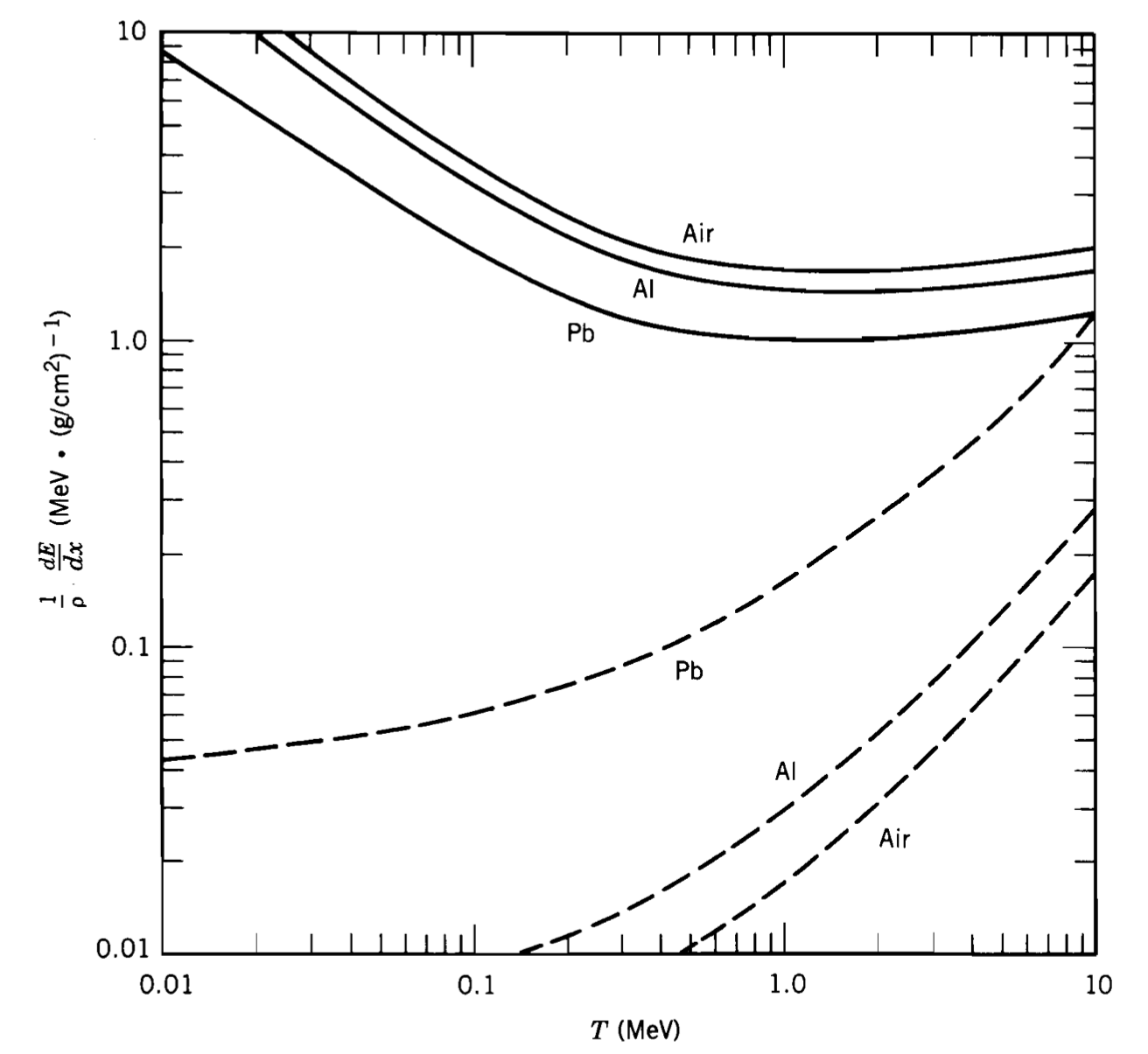
We can take the ratio between the radiation and collision energy losses to get a better idea of the relative contributions from the above two processes. This indicates that the radiative term is significant only at high energy and in ‘heavy’ materials. The adjoining figure shows the energy loss for several materials; solid lines are for collisions, and dashed lines are for radiation.

\[ \dfrac{\left( dE/dx\right) _{r}}{\left(dE/dx\right) _{c}}\approx \lr{\dfrac{T}{m_e c^{2}}+1}\times \dfrac{Z}{1600} \tag{10.8}\]

10.3 Photons

Figure 10.8: General light–matter interactions

Let’s now discuss how electromagnetic radiation (i.e. photons) interacts with matter. Light interacts with matter through many processes (Rayleigh, Mie, Raman, Fluorescence,\(\ldots\)). In this section, I will only focus on high-energy photons (\(\gamma\) and X-rays) as these are more common in nuclear reactions. There are three possible processes (shown in the adjoining figure) we need to consider:

Photoelectric Effect where photons are absorbed and photoelectrons emitted.
Compton Scattering where photons scatter off electrons, change ‘colour’ and the electrons rush away with kinetic energy stolen from the photons.
Pair production where a photon is converted into a particle-antiparticle pair.

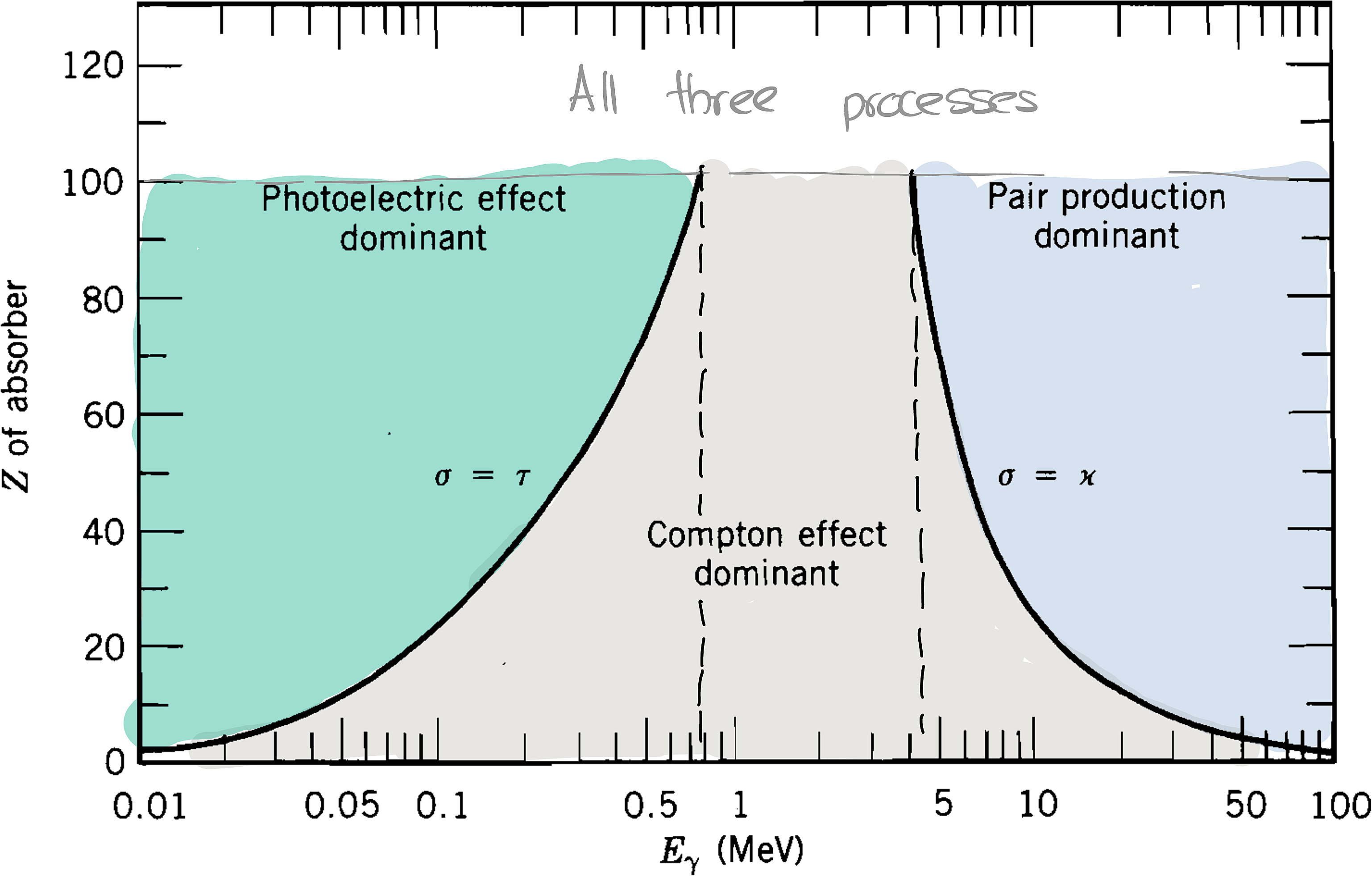
Figure 10.9: Dominant photon-interaction regions

The figure on the right, shows the various energy and \(Z\) regimes in which each process dominates. You can see that the photoelectric effect dominates at low energies (below about 500 keV) and pair production at higher (more than about 5 MeV) energies. \(\tau\) and \(\kappa\) are the linear attenuation coefficients (see ?exm-beer-lambert and ?eq-beer-lambert-2) for these processes that we will soon discuss. NIST maintains the XCOM database that has cross-sections for all these processes.

Before we move on, note that all these processes need the electrons to be bound (i.e. not free) because energy and momentum conservation prevent a photon from interacting with a free electron.

10.3.1 Photoelectric Effect

The photoelectric effect involves the absorption of a photon and the subsequent emission of a (photo) electron. Einstein was awarded the Nobel Prize in Physics in 1921 for his explanation of the photoelectric effect, which is based on the following equation:

\[ T_e = E_\gamma - B_e \tag{10.9}\]

\(B_e\) is the binding energy of the electron, \(T\) the kinetic energy and \(E_\gamma\) the energy of the photon. For this process to proceed, the photon must have more energy than \(B_e\).

We don’t have an expression to calculate the photoelectric cross-sections. However, we have experimental data (e.g. from the NIST database) which indicate that the cross-section increases as \(Z^4\) for low energy (< 100 keV) photons and that the cross-section generally decreases (rapidly) with energy as \(E_\gamma^{-3}\).

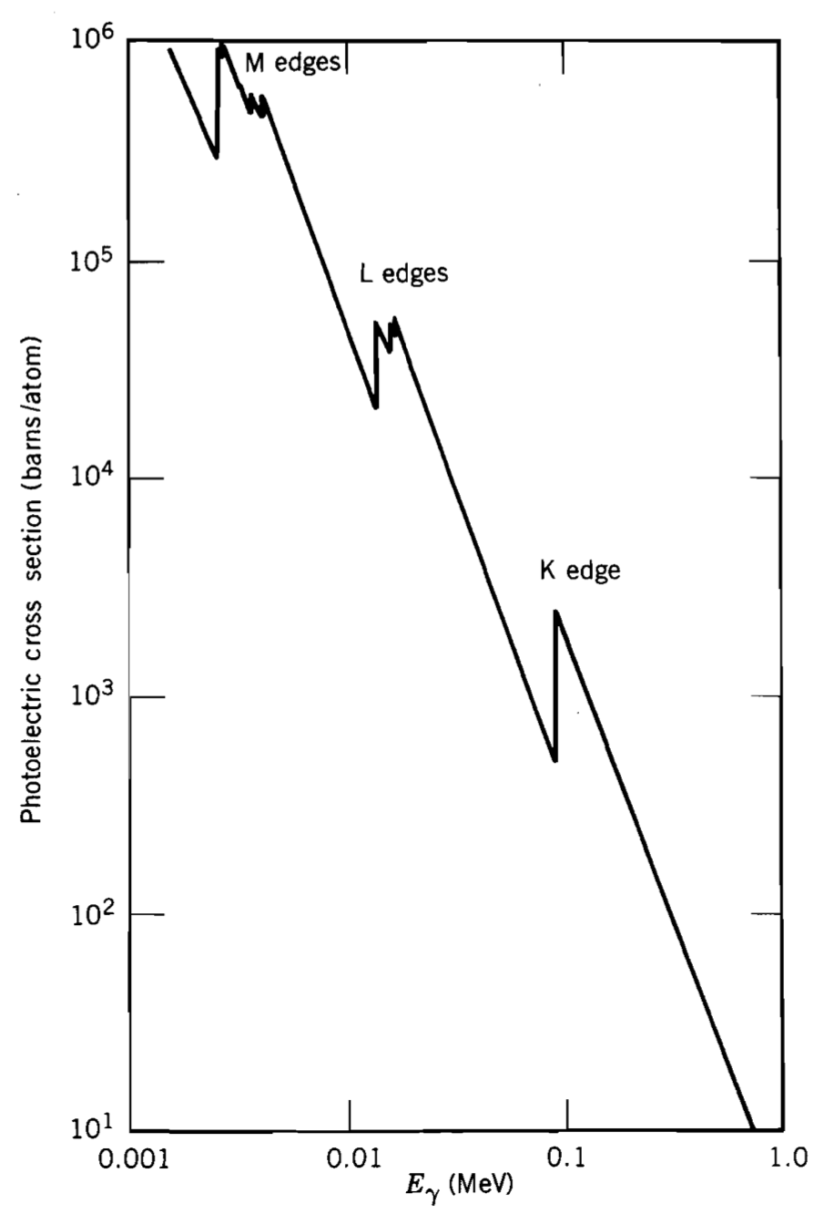
Figure 10.10: Photoelectric absorption edges

There are characteristic abrupt jumps in the cross-sections because the photons with more energy can release electrons from deeper shells. These are called (K, L, M…) absorption edges. You can see these in the adjoining figure.

Unless the interaction occurs near the surface, the material will reabsorb all the photoelectrons. Additionally, the excited atom left behind needs to capture an electron and relax back to the ground state. This can involve the emission of an x-ray photon or, sometimes, another (low energy) electron through a process called Auger emission. The former dominates for low-\(Z\) elements, while the latter is more common for high-\(Z\) elements.

10.3.2 Compton scattering

In 1923, Arthur Compton performed a photon-electron collision experiment in which a photon scatters from an atomic electron resulting in a less energetic (longer wavelength) photon and a scattered electron carrying the energy lost by the photon. This experiment convinced people of the existence of the photon and Einstein’s explanation of the photoelectric effect. The Compton effect is modelled as a photon interacting with a nearly free electron because of the large energy disparity between the impinging photon and the electron rest energy.

Kinematics

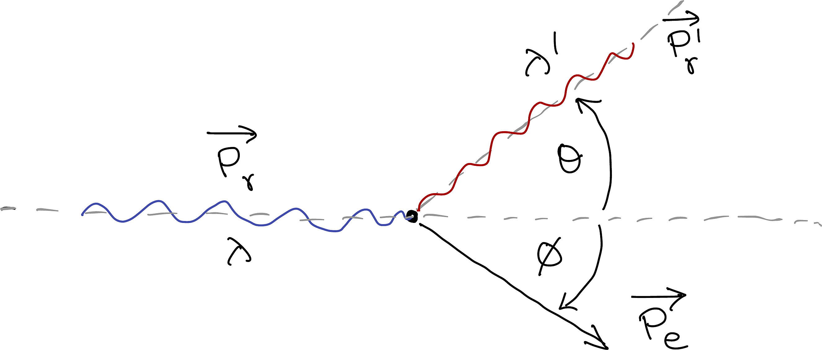
Let’s work out the kinematics of Compton Scattering. Our analysis must be relativistic because the energies involved are comparable to the electron’s rest energy \(0.511\) MeV.

We want to determine the energy of the outgoing photon (i.e. we need to get \(p_\gamma'\)).

The energy and momentum of a photon of wavelength, \(\lambda\) is given by: \[ \begin{array}{ccr} p_\gamma = \dfrac{h}{\lambda} & \text{and} & E_\gamma = p_\gamma c \end{array} \]

Since momentum is conserved:

\[ \v{p_{\gamma}}=\v{p_{\gamma}'}+\v{p_{e}} \tag{10.10}\]

Since energy is conserved:

\[ \begin{align} E_{\gamma} + m_ec^2 &=E_{\gamma}'+E_{e}\\ \ie p_{\gamma}c+ m_ec^2&=p_{\gamma}'c+E_{e} \end{align} \tag{10.11}\]

Further, we know that the electron must abide by:

\[ E_e^2 = p_e^2c^2 + m_e^2c^4 \tag{10.12}\]

From Equation 10.10:

\[\begin{align} \v{p_e} &= \v{p_\gamma} - \v{p_\gamma'}\\ \Rightarrow p_e^2 &= (\v{p_\gamma} - \v{p_\gamma'}) \cdot (\v{p_\gamma} - \v{p_\gamma'})\\ &= p_\gamma^2 + {p_\gamma'}^{2} - 2\v{p_\gamma} \cdot \v{p_\gamma'} \\ &= p_\gamma^2 + {p_\gamma'}^{2} - 2p_\gamma p_\gamma' \cos{\theta} \end{align}\]

From Equation 10.11:

\[\begin{align} E_e &= c(\p-\pp) + mc^2 \\ \Rightarrow E_e^2 &= c^2(\p-\pp)^2 + 2 mc^3(\p-\pp) + m^2c^4 \\ \end{align}\]

Substituting these in Equation 10.12:

\[ \begin{align} \left[c^2(\p-\pp)^2 + 2 m_e c^3(\p-\pp) + m_e^2c^4\right] &= \left[\p^2 + {\pp}^{2} - 2\p \pp \cos{\theta}\right]c^2 + m_e^2c^4 \\ \ie \left[(\p-\pp)^2 + 2 m_e c(\p-\pp) + \cancel{m_e^2c^2}\right] &= \left[\p^2 + {\pp}^{2} - 2\p \pp \cos{\theta}\right] + \cancel{m_e^2c^2} \\ \ie (\p^2+\pp^2 - 2\p\pp) + 2 m_e c(\p-\pp) &= \p^2 + {\pp}^{2} - 2\p \pp \cos{\theta} \\ \ie (\cancel{\p^2}+\cancel{\pp^2} - 2\p\pp) + 2 m_e c(\p-\pp) &= \cancel{\p^2} + \cancel{\pp^2} - 2\p \pp \cos{\theta} \\ \ie \p\pp - m_e c(\p-\pp) &= \p \pp \cos{\theta} \\ \Rightarrow m_e c(\p-\pp) &= \p \pp(1-\cos{\theta}) \\ \Rightarrow \dfrac{1}{\pp}-\dfrac{1}{\p} &= \dfrac{1}{m_ec}(1-\cos{\theta}) \\ \ie \dfrac{1}{h/\lambda'}-\dfrac{1}{h/\lambda} &= \dfrac{1}{m_ec}(1-\cos{\theta}) \\ \therefore \lambda'-\lambda &= \dfrac{h}{m_ec}(1-\cos{\theta}) \\ \end{align} \]

\[ \lambda' = \lambda + \lambda_0(1-\cos{\theta}) \tag{10.13}\]

Where, \[ \lambda_0= \dfrac{h}{m_ec} \]

Differential scattering cross-section

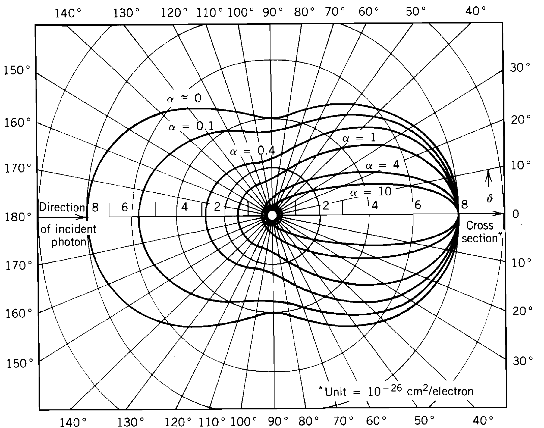
Klein-Nishina worked on a quantum mechanical treatment of the Compton scattering to yield the following Klein-Nishina formulae:

\[ \da{\sigma_c}{\Omega}=r_{0}^{2}\bigg[ \dfrac{1}{1+\alpha \left( 1-\cos \theta \right) }\bigg ]^{2} \bigg[ \dfrac{1+\cos^2 \theta }{2}\bigg ] \bigg[ 1+\dfrac{\alpha ^{2}\left( 1-\cos\theta \right) ^{2}}{\left( 1+\cos ^{2}\theta \right) \left( 1+\alpha \left( 1-\cos \theta \right) \right) }\bigg ] \tag{10.14}\]

\[ \sigma _{c}=\dfrac{\pi r_{0}^{2}}{\alpha } \left\{ \left[ 1-\dfrac{2 \left( \alpha +1\right) }{\alpha ^{2}}\right]\, \ln \left( 2\alpha +1\right) +\dfrac{1}{2}+\dfrac{4}{\alpha }-\dfrac{1}{2 \left( 2\alpha +1\right) ^{2}} \right\} \tag{10.15}\]

Where:

\(\theta\)	Scattering angle of the photon
\(\da{\sigma_c}{\Omega}\)	Differential scattering cross section
\(E_\gamma\)	Original energy of the phtotn
\({E'}_g\)	Energy of the scattered photon
\(r_0=\f{e^2}{4\pi\epsilon_0\, m_e c^2}\)	Classical electron radius (\(\approx 2.881\) fm)
\(\alpha = \f{E_\gamma}{m_e c^2}\)	Photon energy in units of electron rest energy

Note that you can derive Equation 10.15 by integrating Equation 10.14 overall \(\theta\). Further, these cross-sections are per electron. So, if you want the Compton scattering cross-section for the material, you have to use the atomic number (\(Z\)) and the number of atoms per unit volume (\(n\)) as follows:

\[ \sigma = \sigma_c n Z \tag{10.16}\]

The following is a polar plot of the differential cross section for Compton scattering.

Figure 10.12: Klein–Nishina angular distribution

10.3.3 Pair Production

The third process that photons can participate in is pair production, where a photon creates an electron-positron pair:

\[ \me{\gamma}{e^-+e^+} \]

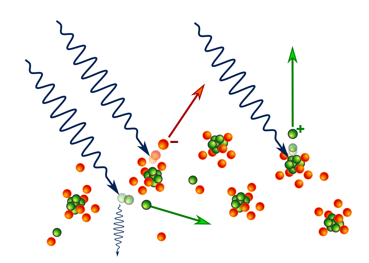
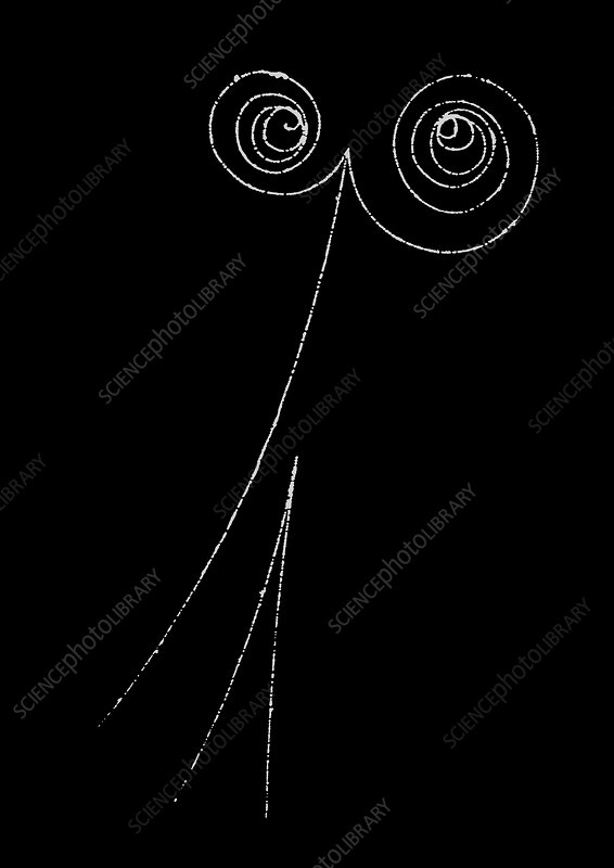
The above bubble chamber photograph from Science Photo Library (sciencephoto.com) shows the production of two electron-positron pairs. Two invisible gamma-ray photons enter at the top, each producing an electron-positron pair. One of the incoming photons also displaces an atomic electron, which shoots off towards the bottom.

There is obviously a threshold of \(2m_e c^2\) for this process to occur. However, pair production is dominant only for energies above 5 MeV. The energetics of the process can be given by: \[ E_\gamma = T_+ + m_e c^2 + T_- + m_e c^2 \]

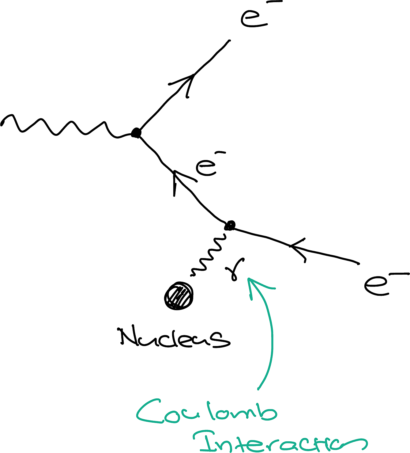
Where the \(T\)’s are the energies of the electron and positron. Like, the photoelectric effect, pair production requires the presence of a massive atom for momentum conservation. However, the subsequent recoil energy of the nucleus is negligible compared to other terms in the above equation. More specifically, pair production can proceed in the Coulomb field of the nucleus or the Coulomb field of an atomic electron. The cross-sections for these two processes are different. The adjoining figure shows a Feynman diagram for pair production.

Figure 10.13: Pair-production photograph

Figure 10.14: Pair-production Feynman diagram

10.3.4 Attenuation

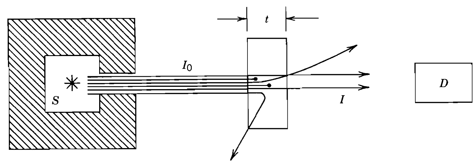
Figure 10.15: Photon attenuation geometry

Consider the situation depicted in the above figure where a highly collimated beam of monoenergetic photons are incident on a slab of thickness \(t\). Since all three processes we discussed can come into play and remove photons from the original beam, those that arrive at the detector have not interacted and have the same original energy. This is sometimes called an all or nothing interaction. This differs from charged particles, where you get the same number coming through (of course, depending if \(t\) is less than the range) but with diminished energies.

To describe this process quantitatively, we use the total linear attenuation coefficient (\(\mu\)), which is the total probability per unit length, for the removal of a photon.

\[ \mu = \tau + \sigma + \kappa \tag{10.17}\]

Where \(\tau\), \(\sigma\) and \(\kappa\) are related to the probability of the process for unit length for the photoelectric effect, Compton scattering (Equation 10.16) and pair production, respectively. We previously discussed this concerning the Beer-Lambert law (Equation 9.10) which we can now use here to get:

\[ I = I_0 e^{-\mu t} \]

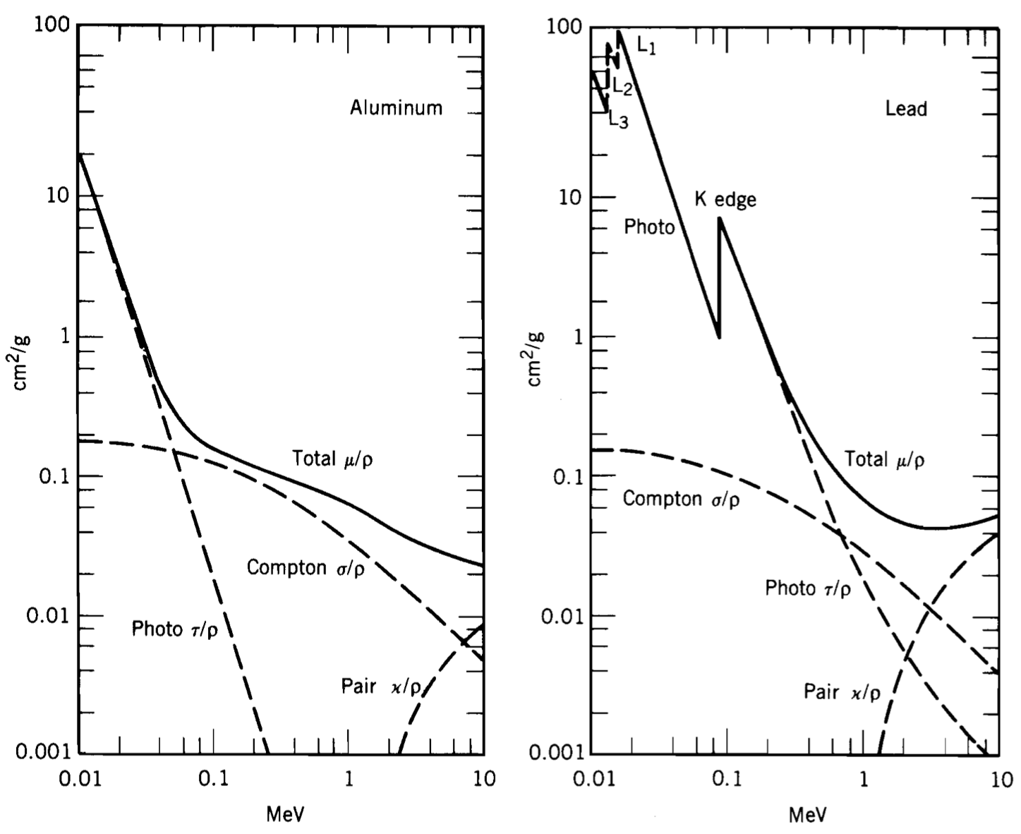
Sometimes we want to compare the contributions of each of the three processes in various elements. However, since different elements have different numbers of electrons, the experimentally measured values will correspondingly change. For example, lead (Pb) with more electrons than aluminium will have more events of Compton scattering. To account for this, we also have a photon mass attenuation coefficient which we get by dividing the linear attenuation coefficients by the density. The following plot shows these coefficients for Al and Pb.

Figure 10.16: Photon mass attenuation coefficients

Chapter References

Particle Data Group et al. Review of Particle Physics. Progress of Theoretical and Experimental Physics 2022, 083C01 (2022).