6 Lifetimes, Decays and Respnances
\[ \newcommand\v[1]{\boldsymbol{#1}} \newcommand\vdot[2]{\v{#1}\cdot\v{#2}} \]
\[ \newcommand{\dd}[2][]{\mathrm{d}^{#1}#2} \]
\[ \newcommand\f[2]{\dfrac{#1}{#2}} \newcommand\da[2]{\dfrac{d #1}{d #2}} \newcommand\daa[2]{\dfrac{d^2 #1}{d #2^2}} \newcommand\pa[2]{\dfrac{\partial #1}{\partial #2}} \newcommand\pal[3]{\left.\dfrac{\partial #1}{\partial #2}\right|_{#3}} \newcommand\paa[2]{\dfrac{\partial^2 #1}{\partial #2^2}} \newcommand\pab[3]{\dfrac{\partial^2 #1}{\partial #2 \partial #3}} \def\half{\frac{1}{2}} \]
\[ \newcommand\ket[1]{\left|#1\right\rangle} % |x> \newcommand\exp[1]{\left\langle#1\right\rangle} % <x> \newcommand\lr[1]{\left(#1\right)} % (x) \newcommand\lrs[1]{\left[#1\right]} % [x] \newcommand\lra[1]{\left|#1\right|} % |x| \newcommand\lrc[1]{\left\{#1\right\}} % {x} \newcommand\lrl[3]{\left.#1\right|_{#2}^{#3}} % x_limits \]
\[ \def\ie{\text{i.e.}\quad} \]
\[ \newcommand{\me}[3][\rightarrow]{{#2}#1{#3}} % Typical reaction \newcommand{\nr}[3]{{#1}\,({#2})\,{#3}} % Nuclear reactions \newcommand{\ele}[4]{_{#2}^{#3}{\textbf{#1}}_{#4}} \newcommand{\el}[2]{^{#2}\text{#1}} \newcommand{\til}[2][\mathbf{\sim}]{\underset{#1}{{#2}}} \newcommand{\b}[1]{\overline{#1}} \]
\[ \newcommand{\coulomb}[1]{\dfrac{#1}{4\pi\epsilon_0}} \def\degree{^*} \]
\[ \def\amu{\text{ amu}} \def\J{\text{ J}} \def\K{\text{ K}} \def\s{\text{ s}} \def\second{\text{ s}} \def\Psecond{\text{ s}^{-1}} \def\m{\text{ m}} \def\mm{\text{ mm}} \def\km{\text{ km}} \def\fm{\text{ fm}} \def\mum{\text{ $\mu$m}} \def\mus{\text{ $\mu$s}} \def\mPERs{\text{ ms$^{-1}$}} \def\eV{\text{ eV}} \def\keV{\text{ keV}} \def\GeV{\text{ GeV}} \def\MeV{\text{ MeV}} \def\MeVc{\text{ MeV/c$^2$}} \def\KeVc{\text{ KeV/c$^2$}} \newcommand\ttp[1]{\times 10^{#1}} % To The Power \]
\[ \def\en{\nu_e} \def\Aen{\b{\nu_e}} \def\mun{\nu_\mu} \def\Amun{\b{\nu}_\mu} \]
\[ \def\uraniumA{\ele{U}{92}{233}{}} \def\uraniumB{\ele{U}{92}{235}{}} \def\uraniumC{\ele{U}{92}{238}{}} \def\carbonB{\ele{C}{6}{14}{}} \def\nitrogenB{\ele{N}{7}{14}{}} \def\oxygenA{\ele{O}{8}{14}{}} \def\oxygenB{\ele{O}{8}{16}{}} \]
\[ % \def\com{\text{\scriptsize CM}} \def\com{\mathrm{\scriptsize CM}} \]
\[ \def\l{l} \]
\[ \def\g{\gamma} \]
What to Expect in This Chapter
A striking feature of many subatomic particles is their tendency to decay spontaneously. Although we cannot predict when any individual particle will decay, we can describe the behaviour of a large collection of particles with remarkable precision.
In this we will develop the concepts of decay rate and lifetime and examine how they are related. We will then use a simple quantum-mechanical model to show how a particle’s finite lifetime leads naturally to a spread in its measured energy or mass(the Breit–Wigner distribution).
Along the way, I will introduce several new concepts, including decay width and phase space. Some of these ideas will be developed more fully in later chapters. For now, the goal is to understand why they arise, what physical questions they answer, and how they fit into our description of particle decay.
6.1 Patterns in Particle Decays
6.1.1 Branching Ratios & Decay Widths
A particle can often decay through several different modes. For example, consider the charged kaon, \(K^+\). Some of its possible decay modes are shown below:
\[ \begin{array}{rclc} \me[&\rightarrow&]{K^+}{\mu^+ + \nu_\mu} & (64\%)\\ \me[&\rightarrow&]{K^+}{\pi^+ + \pi^0} & (21\%)\\ \me[&\rightarrow&]{K^+}{\pi^+ + \pi^+ + \pi^-} & (6\%)\\ \me[&\rightarrow&]{K^+}{\pi^0 + e^+ + \nu_e} & (5\%) \end{array} \tag{6.1}\]
The percentages associated with these modes are called branching ratios. A large branching ratio means that a large fraction of the particles decay through that particular mode, while a small branching ratio means that the mode occurs less frequently.
The percentages associated with these modes are called branching ratios. A large branching ratio means that a large fraction of the particles decay through that particular mode, while a small branching ratio means that the mode occurs less frequently.
Another way to describe particle decay is through its decay width, denoted by \(\Gamma\). Each decay mode is assigned a partial decay width, \(\Gamma_i\), while the sum of all the partial widths gives the total decay width:
\[ \Gamma_{\text{total}}=\sum_i\Gamma_i. \tag{6.2}\]
The branching ratio for a particular mode is the ratio of its partial decay width to the total decay width:
\[ \operatorname{BR}_i = \frac{\Gamma_i}{\Gamma_{\text{total}}}. \tag{6.3}\]
We will develop these ideas later. For the moment, let us become familiar with the language and terminology of particle decays.
One of the goals of nuclear and particle physics is to calculate these branching ratios theoretically and measure them experimentally.
6.1.2 Some rules of thumb
Another conspicuous feature of particle decay is that particle lifetimes span an extraordinarily broad range, about 28 orders of magnitude! How quickly a decay proceeds depends strongly on the interaction responsible for it.
Table 6.1 provide a useful rule of thumb:
| Interaction | Typical lifetime | Example |
|---|---|---|
| Strong | \(\sim 10^{-23}\,\mathrm{s}\) | \(\me{\Delta^{++}}{p+\pi^+}\) |
| Electromagnetic | \(\sim 10^{-16}\,\mathrm{s}\) | \(\me{\pi^0}{\gamma+\gamma}\) |
| Weak | \(\sim 10^{-13}\,\mathrm{s}\) | \(\me{\Sigma^-}{n+e^-+\bar{\nu}_e}\) |
Another useful rule of thumb is that, for a given interaction, a decay generally proceeds more rapidly when there is a larger mass difference between the original particle(called the parent) and the products (called the daughters). A larger mass difference usually provides more phase space (more on this in a later chapter) for the decay products.
This helps explain why the neutron has such a long lifetime of about 15 minutes, despite decaying through the weak interaction: the mass difference between the neutron and its decay products is very small.
An excellent way to identify patterns in particle lifetimes is to plot lifetime against mass, as shown below.
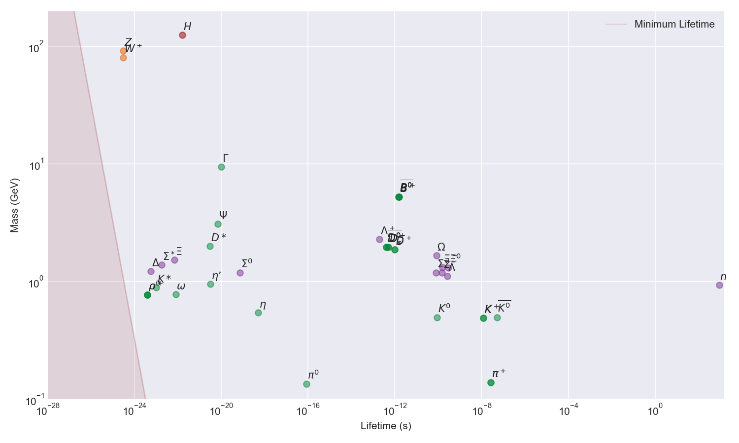
Several patterns are visible in Figure 6.1:
- Particles that decay through the strong interaction tend to cluster at very short lifetimes, typically around \(10^{-23}\,\mathrm{s}\).
- Electromagnetic decays generally have longer lifetimes than strong decays but remain much faster than most weak decays.
- Notice \(\pi^0\) and \(\pi^\pm\): Their masses are similar, but the electromagnetically decaying \(\pi^0\) has a much shorter lifetime than the weakly decaying charged pions.
- The neutron lies at the extreme long-lifetime end of the plot. Although its decay is permitted by the weak interaction, very little energy is available to its decay products, resulting in a strongly suppressed decay rate.
- The \(W^\pm\), \(Z^0\), and Higgs bosons are very massive and decay rapidly because many decay channels are available to them and their decays have substantial phase space.
The broad spread of points shows that there is no simple relationship between mass and lifetime. There are many factors at play such as the interaction involved, the available phase space, the number of accessible decay modes, and any relevant conservation laws or selection rules.
6.2 Lifetimes, Statistically Speaking
A remarkable feature of particle and nuclear decay is that the probability of decay per unit time is constant. That is, provided the particle has survived until the present moment, the probability that it will decay during the next short time interval \(dt\) is \[ \lambda\,dt, \tag{6.4}\]
regardless of whether it has already existed for a nanosecond or for 1,000 years. In this sense, radioactive decay has no memory: an unstable particle does not age, like you and I!
The constant \(\lambda\) is called the decay constant. It represents the probability of decay per unit time.
Let \(P(t)\) be the probability that the particle survives until time \(t\). To survive until \(t+dt\), the particle must first survive until \(t\) and then avoid decaying during the interval \(dt\). Therefore,
\[ P(t+dt)=P(t)\left(1-\lambda\,dt\right). \tag{6.5}\]
Rearranging this expression gives
\[ \frac{P(t+dt)-P(t)}{dt}=-\lambda P(t). \]
In the limit as \(dt\rightarrow 0\), we obtain
\[ \frac{dP}{dt}=-\lambda P. \tag{6.6}\]
With the initial condition \(P(0)=1\), the solution is
\[ P(t)=e^{-\lambda t}. \tag{6.7}\]
This is the familiar exponential decay law.
6.2.1 The Mean Lifetime
Although the decay of an individual particle is unpredictable, but we can calculate the average lifetime of a large collection of identical particles.
The probability that a particle decays between \(t\) and \(t+dt\) is
\[ P(t)(\lambda dt)= \lambda e^{-\lambda t}\,dt =f(t)\,dt, \tag{6.8}\]
where \(f(t)\) is the probability density for the decay time. The mean lifetime is therefore
\[ \begin{aligned} \langle t\rangle &= \int_0^\infty t f(t)\,dt\\ &= \int_0^\infty t\lambda e^{-\lambda t}\,dt\\ &= \frac{1}{\lambda}. \end{aligned} \tag{6.9}\]
We denote this mean lifetime by \(\tau\):
\[ \tau=\langle t\rangle=\frac{1}{\lambda}. \tag{6.10}\]
There is another useful way to understand \(\tau\). Substituting \(t=\tau\) into the survival probability gives
\[ P(\tau) = e^{-\lambda\tau} = e^{-1}=\approx 0.37. \]
In other words, after one lifetime, about \(37\%\) of the original particles remain. Notice that \(\tau\) is not the time at which every particle has decayed—it is a statistical quantity.
6.2.2 A Collection of Particles
If we begin with \(N_0\) identical unstable particles; since each particle has the same survival probability, the expected number remaining at time \(t\) is
\[ N(t)=N_0P(t). \tag{6.11}\]
Therefore,
\[ N(t)=N_0e^{-\lambda t} =N_0e^{-t/\tau}. \tag{6.12}\]
For a finite sample, the number actually observed will fluctuate around this expected value. For a very large number of particles, however, the measured decay curve closely follows the exponential law we are so used to.
The familiar half-life, \(t_{1/2}\), is the time at which half of the original particles remain:
\[ N(t_{1/2})=\frac{N_0}{2}. \]
It follows that
\[ t_{1/2} = \frac{\ln 2}{\lambda} = \tau\ln 2. \tag{6.13}\]
6.3 Particle Lifetimes, Quantum Mechanically
Let us now build a simple quantum-mechanical model of particle decay. Consider an energy eigenstate \(a\) with wavefunction
\[ \Psi_a(\mathbf{r},t) = \psi_a(\mathbf{r})e^{-iE_at/\hbar}. \tag{6.14}\]
This is a stationary state since:
\[ \left|e^{-iE_at/\hbar}\right|^2=1. \]
So, the system can survive in this state forever.
Suppose instead that the state decays with a characteristic lifetime \(\tau_a\). From our statistical description of decay, its survival probability must decrease as
\[ P_{\mathrm{surv}}(t)=e^{-t/\tau_a}. \]
We can incorporate this behaviour into our quantum-mechanical amplitude by re-writing Equation 6.14 as:
\[ \Psi_a(\mathbf{r},t) = \psi_a(\mathbf{r}) e^{-iE_at/\hbar} \textcolor{darkorange}{e^{-t/(2\tau_a)}}, \qquad t\geq 0. \tag{6.15}\]
Let’s calcuate the probability density by taking the absolute square of the amplitude:
\[ \left|\Psi_a(\mathbf{r},t)\right|^2 = \left|\psi_a(\mathbf{r})\right|^2 e^{-t/\tau_a}. \tag{6.16}\]
If the spatial wavefunction is normalised, then
\[ P(t)\,=\int \left|\Psi_a(\mathbf{r},t)\right|^2\,d^3r = e^{-t/\tau_a}. \]
Here, \(P(t)\) is the probability that the state has survived for a time \(t\) without decaying.
6.3.1 When will the probability occur?
Since, the state must decay at some point we must have that, that the total probaility is one. I.e.
\[ \int P(t)dt = 1 \]
Be careful to distinguish this survival probability from the probability density for the time at which the decay occurs. The decay-time probability density is
\[ w_a(t) = \frac{1}{\tau_a}e^{-t/\tau_a}, \tag{6.17}\]
and it is normalised according to
\[ \int_0^\infty w_a(t)\,dt=1. \]
6.3.2 From Lifetime to Energy Width
There is a price to introducing the factor
\[ e^{-t/(2\tau_a)}. \]
The state no longer has one perfectly defined energy.
Just as position and wave number are related through a Fourier transform, time and angular frequency are also related through a Fourier transform. Since
\[ E=\hbar\omega, \tag{6.18}\]
the Fourier transform of the time-dependent amplitude tells us what combination of energies is needed to describe a decaying quantum state.
Consider the survival amplitude in time:
\[ A_a(t) = e^{-iE_at/\hbar} e^{-t/(2\tau_a)}. \]
Its energy amplitude is proportional to
\[ \begin{align} \widetilde{A}_a(E) &\propto \int_0^\infty e^{iEt/\hbar} e^{-iE_at/\hbar} e^{-t/(2\tau_a)} \,dt\\ &= \int_0^\infty e^\left[ \dfrac{i(E-E_a)t}{\hbar} - \dfrac{t}{2\tau_a} \,dt \right]\\ &\propto \frac{1} {E-E_a+i\Gamma_a/2} \end{align} \tag{6.19}\]
where the decay width is defined by
\[ \Gamma_a \equiv \frac{\hbar}{\tau_a}. \tag{6.20}\]
Taking the absolute square gives the energy probability distribution
\[ P_a(E)\,dE \propto \frac{\Gamma_a\,dE} {(E-E_a)^2+\Gamma_a^2/4}. \tag{6.21}\]
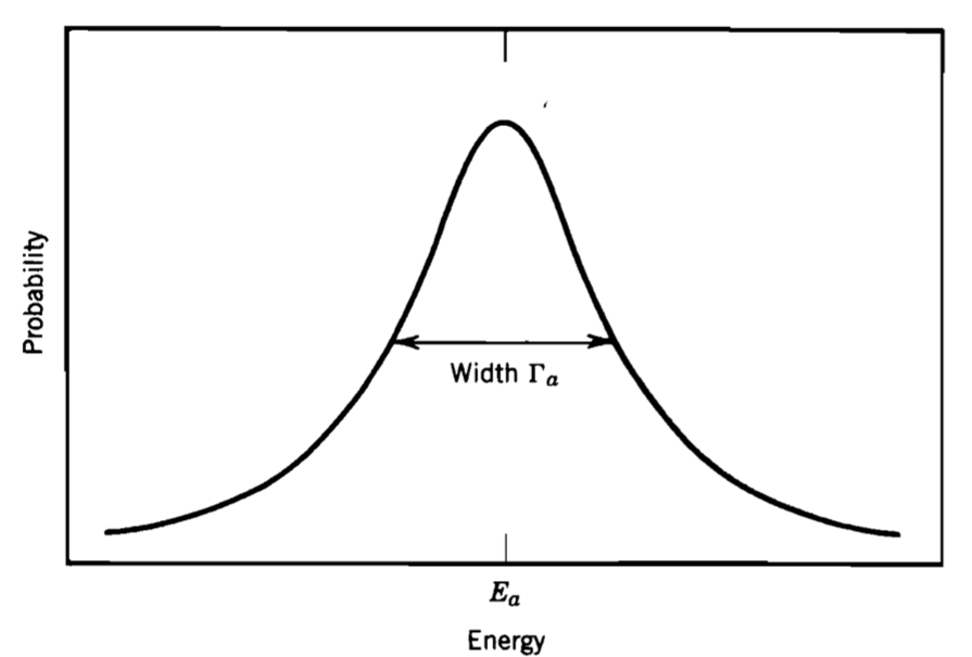
This is called the Breit–Wigner distribution, or the Lorentz distribution.1
The distribution is centred at \(E_a\), and its full width at half maximum (FWHM) is \(\Gamma_a\). Therefore, a short-lived state has a broad energy distribution, while a long-lived state has a narrow energy distribution.
This spread in energy is intrinsic to the unstable state; it is not caused by measurement uncertainty. Even with a perfect detector, repeated measurements would reveal a distribution of energies described by the Breit–Wigner form.
Additionally, I like to point out that the information contained in the Breit–Wigner distribution (see Equation 6.20) is entirely consistent with the energy–time uncertainty relation.
6.4 Not One Mass
One consequence of a particle having a finite lifetime is that its rest mass/energy is not represented by one perfectly sharp value.
Consider the \(\rho(770)\) meson. Althoug it tabulated mass is approximately \(m_\rho \approx 775\,\mathrm{MeV}/c^2\) experimental measurements of its invariant mass produce a range of values rather than a single value. Why is there a range, and how do we choose the quoted mass?
The answer follows from our quantum-mechanical model of decay. Since the \(\rho\) exists for only a very short time, it cannot have a perfectly defined energy. Instead, repeated measurements produce an intrinsic energy distribution described by the Breit–Wigner distribution.
We characterise this distribution using two quantities:
- its central value, which gives the quoted mass of the particle; and
- its FWHM denoted by \(\Gamma\).
For the \(\rho(770)\) meson, these values are approximately
\[ m_\rho \approx 775\,\mathrm{MeV}/c^2, \qquad \Gamma_\rho \approx 150\,\mathrm{MeV}. \]
We can use the width to estimate the lifetime of the \(\rho\):
\[ \tau \approx \f{\hbar}{\Gamma_\rho} = \f{\hbar c}{ \Gamma_\rho c} = \f{197 \MeV\cdot\fm}{150 \MeV\cdot c} = \f{197}{150}\f{10^{-15}\m}{2.997 \times 10^{8} \mPERs} = 4.38\times 10^{-24}\s \]
Thus, the large width of the \(\rho\) is a direct consequence of its extremely short lifetime. Short-lived particles produce broad mass distributions, while long-lived particles produce narrow mass distributions.
6.5 Resonances
6.5.1 What is a resonance?
You will recall that the characteristic timescale for the strong interaction is approximately \(10^{-23}\) s. Consequently, hadrons that decay through the strong interaction are extremely short-lived. Such unstable hadronic states are called resonances, because they behave in some ways like the resonant or excited states encountered in atomic physics.
In this section I like to discuss how these fleeting resonances can be studied experimentally.
6.5.2 Pinning Down Resonances
The strategy used to study resonances relies on an elegant application of special relativity. Let me use a specific example to illustrate how this works.
Suppose we observe the reaction \[ \me{\pi^-+p}{\pi^++\pi^-+n}. \tag{6.22}\]
For each event, we measure the energies and momenta of the outgoing \(\pi^+\) and \(\pi^-\). We can then construct the following Lorentz-invariant quantity
\[ s_{\pi\pi} = (E_{\pi^+}+E_{\pi^-})^2 - ( \v{p}_{\pi^+}+ \v{p}_{\pi^-})^2c^2 \tag{6.23}\]
Based on only reaction 6.23, what will a histogram of \(s_{\pi\pi}\) look like? Since, this involves three products, there are no one way that energy and momentum can be conserved. So, we would expect many different values for s_pipi; meaning we could generally expect a relatively smooth distribution2.
Now suppose instead that the reaction proceeds through a short-lived intermediate state:
\[ \me{\pi^-+p}{\rho^0+n}, \tag{6.24}\]
followed almost immediately by
\[ \me{\rho^0}{\pi^++\pi^-}. \tag{6.25}\]
If the two pions came from the same \(\rho^0\), conservation of four-momentum gives
\[ p_\rho^\mu = p_{\pi^+}^\mu+p_{\pi^-}^\mu. \]
It then follows that
\[ \begin{aligned} s_{\pi\pi} &= (E_{\pi^+}+E_{\pi^-})^2 - ( \v{p}_{\pi^+}+ \v{p}_{\pi^-})^2c^2\\ &= E_\rho^2-\v{p}_\rho^2c^2\\ &= m_{\rho}^2c^4. \end{aligned} \tag{6.26}\]
Whence,
\[ m_{\rho}c^2=\sqrt{s_{\pi\pi}}. \tag{6.27}\]
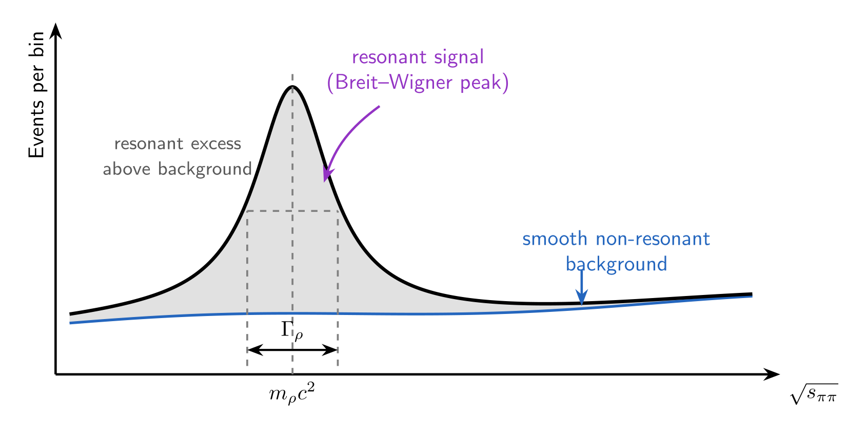
This means that we can reconstruct the mass of the short-lived intermediate state even though the \(\rho^0\) itself is never directly observed. We simply calculate \(\sqrt{s_{\pi\pi}}\) for many events and create a histogram.
The bump in Figure 6.3 corresponds to the \(\rho^0\) resonance. Its central position gives the mass of the \(\rho^0\), while the width of the bump is related to its lifetime.
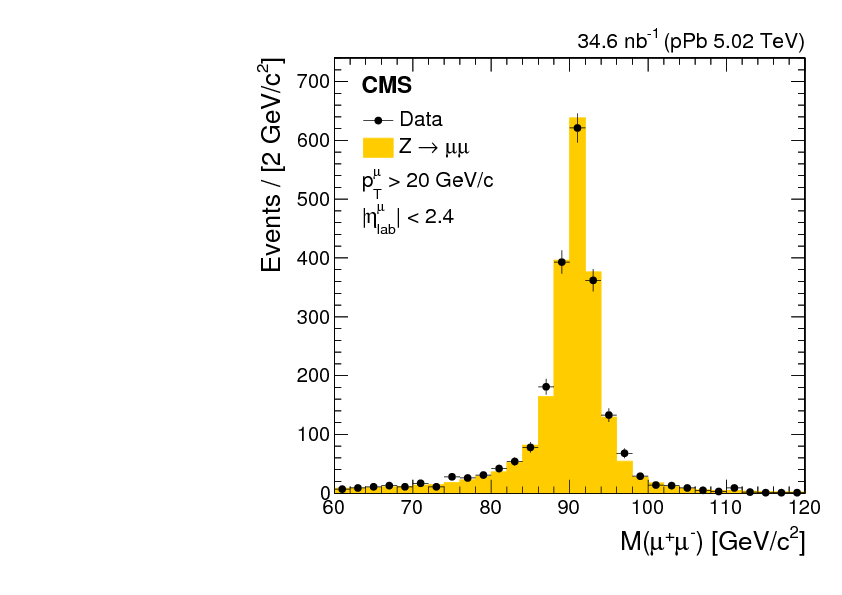
This method is not limited to hadrons. Figure 6.4 shows the invariant-mass distribution of muon pairs measured by the CMS experiment at the LHC. The prominent peak occurs because many of the muon pairs were produced through
\[ \me{Z^0}{\mu^++\mu^-}. \tag{6.28}\]
The \(Z^0\) boson was originally discovered by the UA1 and UA2 experiments at CERN in 1983. The later CMS measurement shown here provides a particularly clear example of how an unstable particle appears as a resonance in the invariant-mass distribution of its decay products.