9 Particle Interactions: Cross Sections
\[ \newcommand\v[1]{\boldsymbol{#1}} \newcommand\vdot[2]{\v{#1}\cdot\v{#2}} \]
\[ \newcommand{\dd}[2][]{\mathrm{d}^{#1}#2} \]
\[ \newcommand\f[2]{\dfrac{#1}{#2}} \newcommand\da[2]{\dfrac{d #1}{d #2}} \newcommand\daa[2]{\dfrac{d^2 #1}{d #2^2}} \newcommand\pa[2]{\dfrac{\partial #1}{\partial #2}} \newcommand\pal[3]{\left.\dfrac{\partial #1}{\partial #2}\right|_{#3}} \newcommand\paa[2]{\dfrac{\partial^2 #1}{\partial #2^2}} \newcommand\pab[3]{\dfrac{\partial^2 #1}{\partial #2 \partial #3}} \def\half{\frac{1}{2}} \]
\[ \newcommand\ket[1]{\left|#1\right\rangle} % |x> \newcommand\exp[1]{\left\langle#1\right\rangle} % <x> \newcommand\lr[1]{\left(#1\right)} % (x) \newcommand\lrs[1]{\left[#1\right]} % [x] \newcommand\lra[1]{\left|#1\right|} % |x| \newcommand\lrc[1]{\left\{#1\right\}} % {x} \newcommand\lrl[3]{\left.#1\right|_{#2}^{#3}} % x_limits \]
\[ \def\ie{\text{i.e.}\quad} \]
\[ \newcommand{\me}[3][\rightarrow]{{#2}#1{#3}} % Typical reaction \newcommand{\nr}[3]{{#1}\,({#2})\,{#3}} % Nuclear reactions \newcommand{\ele}[4]{_{#2}^{#3}{\textbf{#1}}_{#4}} \newcommand{\el}[2]{^{#2}\text{#1}} \newcommand{\til}[2][\mathbf{\sim}]{\underset{#1}{{#2}}} \newcommand{\b}[1]{\overline{#1}} \]
\[ \newcommand{\coulomb}[1]{\dfrac{#1}{4\pi\epsilon_0}} \def\degree{^*} \]
\[ \def\amu{\text{ amu}} \def\J{\text{ J}} \def\K{\text{ K}} \def\s{\text{ s}} \def\second{\text{ s}} \def\Psecond{\text{ s}^{-1}} \def\m{\text{ m}} \def\mm{\text{ mm}} \def\km{\text{ km}} \def\fm{\text{ fm}} \def\mum{\text{ $\mu$m}} \def\mus{\text{ $\mu$s}} \def\mPERs{\text{ ms$^{-1}$}} \def\eV{\text{ eV}} \def\keV{\text{ keV}} \def\GeV{\text{ GeV}} \def\MeV{\text{ MeV}} \def\MeVc{\text{ MeV/c$^2$}} \def\KeVc{\text{ KeV/c$^2$}} \newcommand\ttp[1]{\times 10^{#1}} % To The Power \]
\[ \def\en{\nu_e} \def\Aen{\b{\nu_e}} \def\mun{\nu_\mu} \def\Amun{\b{\nu}_\mu} \]
\[ \def\uraniumA{\ele{U}{92}{233}{}} \def\uraniumB{\ele{U}{92}{235}{}} \def\uraniumC{\ele{U}{92}{238}{}} \def\carbonB{\ele{C}{6}{14}{}} \def\nitrogenB{\ele{N}{7}{14}{}} \def\oxygenA{\ele{O}{8}{14}{}} \def\oxygenB{\ele{O}{8}{16}{}} \]
\[ % \def\com{\text{\scriptsize CM}} \def\com{\mathrm{\scriptsize CM}} \]
\[ \def\l{l} \]
\[ \def\g{\gamma} \]
What to Expect in This Chapter
So far, we have mainly discussed what can happen when two particles interact. For example, an electron and a positron can annihilate. But if we direct 1000 electrons towards 1000 positrons, will all of them annihilate? If not, how many interactions should we expect?
To answer questions such as these, we need a probabilistic description of particle interactions. The central quantity is the cross-section. It connects the underlying interaction physics to quantities that can be measured experimentally, such as the number of events recorded by a detector.
These ideas are invaluable because much of our knowledge of nuclei, particles, atoms and molecules comes from directing a beam at a target and observing what emerges. Think of Rutherford scattering, particle colliders and fluorescence spectroscopy.
By the end of this chapter, you should be able to interpret total, partial and differential cross-sections and connect them to attenuation, event rates and the mean free path.
9.1 The Idea of a Cross-Section
A cross-section tells us how likely it is for a specified interaction or outcome to occur under some experimental conditions.
For example, in a Rutherford-style experiment we might ask:
- How frequently does an \(\alpha\) particle interact with a gold nucleus?
- How frequently is it scattered into a particular range of angles?
- How frequently does a particular reaction channel occur?
9.2 A Simple Geometrical Model
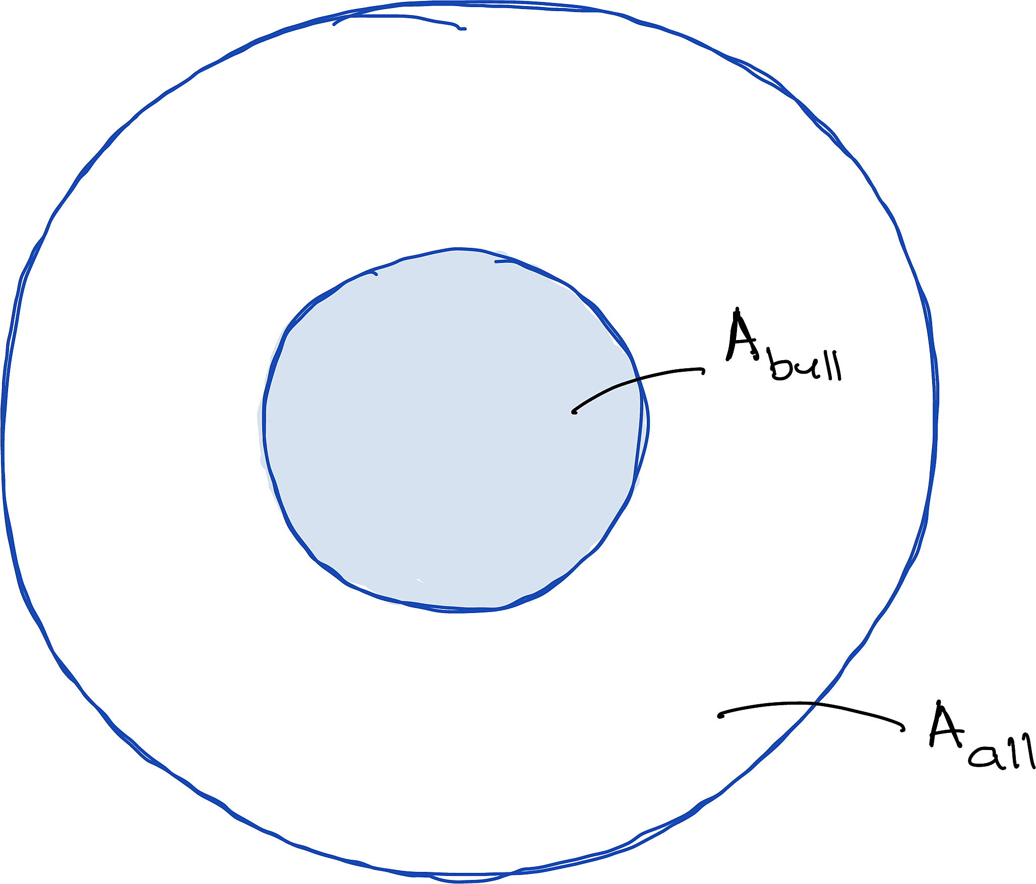
Imagine throwing a large number of darts uniformly and randomly at a board. If \(N_0\) darts land somewhere on the board and \(N_{\text{bull}}\) land inside the bull’s-eye, then it is reasonable to expect that
\[ \frac{N_{\text{bull}}}{N_0} \approx \frac{A_{\text{bull}}}{A_{\text{board}}}. \tag{9.1}\]
The larger the bull’s-eye, the greater the probability of a hit. This gives us our first geometrical picture of a cross-section: it behaves like a target area.
This analogy is useful as a starting point, but it should not be taken too literally. In nuclear and particle physics, \(\sigma\) can depend on many factors(e.g. particle energies, spins and the dynamics of the interactions, quantum interference). A cross-section is therefore not necessarily the physical size of a particle or nucleus. It is an effective area that represents the probability of a particular interaction or outcome.
9.2.1 Units
Since a cross-section has dimensions of area, it is measured in units of area. The unit commonly used in nuclear and particle physics is the barn:
\[ 1\,\mathrm{b}=10^{-28}\,\mathrm{m^2}. \]
Commonly used submultiples of the barn are:
| Unit | Symbol | Equivalent |
|---|---|---|
| millibarn | \(\mathrm{mb}\) | \(10^{-3}\,\mathrm{b}\) |
| microbarn | \(\mu\mathrm{b}\) | \(10^{-6}\,\mathrm{b}\) |
| nanobarn | \(\mathrm{nb}\) | \(10^{-9}\,\mathrm{b}\) |
| picobarn | \(\mathrm{pb}\) | \(10^{-12}\,\mathrm{b}\) |
9.3 From One Interaction Centre to a Target
9.3.1 A Single Centre
I will now use a light-hearted, ‘happy’ model to further develop the ideas of cross-sections further. But don’t worry, I will make it more serious later.
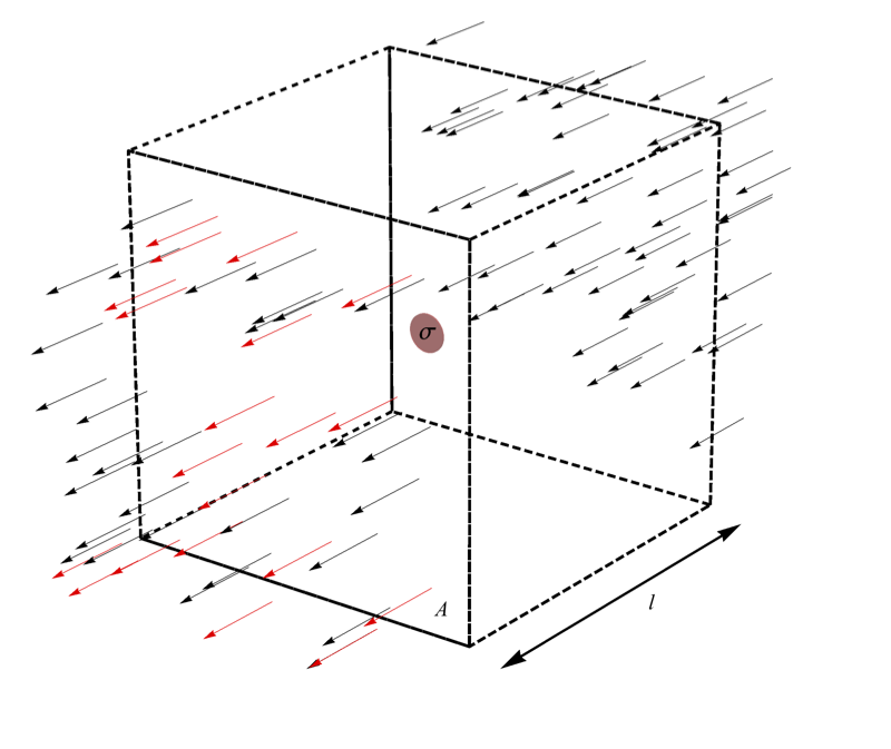
Suppose projectiles pass through an area \(S\) containing one “happiness centre”. A projectile that interacts with the centre becomes happy. Let the centre have an effective happiness cross-section \(\sigma\).
If the incident projectiles are distributed uniformly across the area, then
\[ \frac{N_{\mathrm{int}}}{N_0} = \frac{\sigma}{S}, \tag{9.2}\]
where \(N_{\mathrm{int}}\) is the number of projectiles that interact and “become happy”. The crucial point is that all the complicated interaction physics is encapsulated in \(\sigma\). If we have a sufficiently developed theory, we may calculate \(\sigma\) from first principles. Otherwise, we can determine it experimentally. Comparing the theoretical prediction with the measured value provides an important test of the theory.
9.3.2 Many Centres: The Thin-Target Approximation
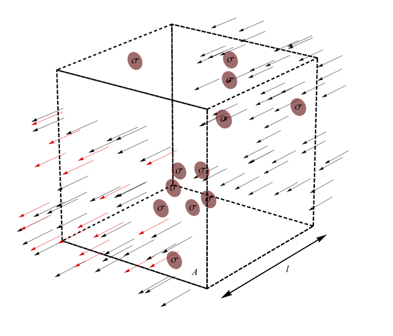
Now suppose that the sample contains many interaction centres with number density \(n\). If the sample has cross-sectional area \(S\) and thickness \(l\), its volume is \(Sl\). The total number of interaction centres is therefore
\[ N_{\text{centres}}=nSl. \]
Provided the target is sufficiently thin that the beam is not substantially attenuated and the probability of multiple interactions is negligible, we can treat each centre as an independent opportunity for interaction.
\[ \begin{aligned} \frac{N_{\mathrm{int}}}{N_0} &= \frac{\sigma}{S}N_{\text{centres}}\\ &= \frac{\sigma}{S}(nSl)\\ &= n\sigma l. \end{aligned} \tag{9.3}\]
Thus,
\[ {N_{\mathrm{int}}=N_0n\sigma l} \qquad (n\sigma l\ll1). \tag{9.4}\]
The quantity \(nl\) is the areal number density and has units of interaction centres per unit area. The product \(n\sigma l\) is dimensionless and represents the interaction probability in the thin-target limit.
If the material has mass density \(\rho\) and molar mass \(M\), then
\[ n=\frac{N_A\rho}{M}, \tag{9.5}\]
so that
\[ \frac{N_{\mathrm{int}}}{N_0} \approx \frac{N_A\rho\sigma l}{M}. \tag{9.6}\]
Here, \(N_A\) is the Avogadro constant.
9.4 Attenuation Through a Thick Target
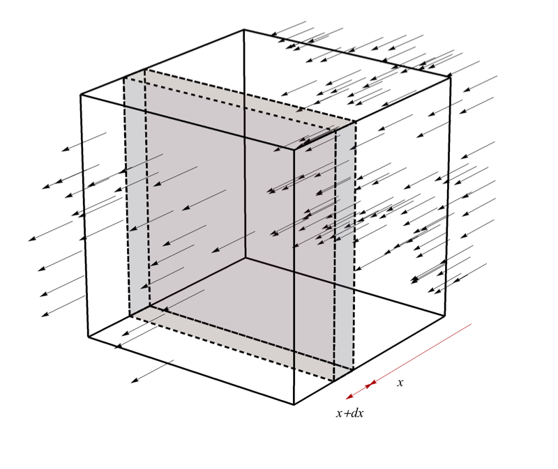
The approximation in Equation 9.4 cannot remain valid as the target becomes thick. Let us now develop a more general result that accounts for the attenuation of the beam as it passes through the target.
Let \(N(x)\) be the number of particles that have travelled a distance \(x\) without undergoing the specified interaction. Within the next thin layer of thickness \(dx\), the change in this number is
\[ dN=-N(x)n\sigma\,dx. \tag{9.7}\]
The negative sign indicates that the number of surviving particles decreases with distance. Rearranging gives
\[ \frac{dN}{N}=-n\sigma\,dx. \]
Integrating from \(N_0\) at \(x=0\) to \(N(x)\) at depth \(x\) gives
\[ \int_{N_0}^{N(x)}\frac{dN'}{N'} = -n\sigma\int_0^x dx', \]
and hence
\[ {N(x)=N_0e^{-n\sigma x}}. \tag{9.8}\]
The number of particles that have undergone the specified interaction is
\[ N_{\mathrm{int}}(x)=N_0-N(x). \]
Therefore, the fraction that has interacted is
\[ { \frac{N_{\mathrm{int}}(x)}{N_0} = 1-e^{-n\sigma x} }. \tag{9.9}\]
For a thin target, \(n\sigma x\ll1\), and
\[ e^{-n\sigma x}\approx1-n\sigma x. \]
The exact result then reduces to
\[ \frac{N_{\mathrm{int}}}{N_0}\approx n\sigma x, \]
recovering the thin-target approximation.
9.4.1 Beer–Lambert Law
For photons passing through an absorbing medium, we may write the same result in terms of intensity:
\[ I(x)=I_0e^{-\mu x}, \tag{9.10}\]
where
\[ \mu=n\sigma \tag{9.11}\]
is the linear attenuation coefficient. In practice, \(\sigma\) generally depends on the photon wavelength or energy and must include all the processes that remove photons from the measured beam.
This exponential attenuation relationship is commonly known as the Beer–Lambert law. It plays an important role in photon-absorption and attenuation measurements, particularly in spectroscopy and analytical chemistry.
9.5 Total and Partial Cross-Sections
A given initial state may lead to several mutually exclusive outcomes or channels. If \(\sigma_i\) is the partial cross-section for channel \(i\), then
\[ { \sigma_{\mathrm{total}} = \sum_i\sigma_i }. \tag{9.12}\]
For example, the total cross-section may contain elastic scattering, inelastic scattering and reaction channels. We must specify which processes are included whenever we quote a “total” cross-section.
The fraction of interactions that proceeds through channel \(i\) is
\[ \frac{\sigma_i}{\sigma_{\mathrm{total}}}. \tag{9.13}\]
This resembles a decay branching ratio we encountered previously, although cross-sections are related to collision probabilities rather than decay probabilities.
9.6 Differential Cross-Sections
A cross-section associated with a particular channel usually includes many possible ways in which that outcome can occur. For example, \(\sigma_{\mathrm{elastic}}\) tells us how frequently particles scatter elastically, but it does not tell us how those particles are distributed in scattering angle.
Often, we need this more detailed information rather than only the total cross-section for the channel. We therefore introduce a differential cross-section, which describes how the cross-section is distributed with respect to a measurable quantity, such as scattering angle or outgoing-particle energy. Integrating the differential cross-section over the allowed values of that quantity gives the corresponding total cross-section.
9.6.1 Differential Cross-Sections w.r.t. \(X\)
Suppose \(X\) is an observable. For a thin target, the number of events with values between \(X\) and \(X+dX\) can be expressed as: \[ dN = N_0nl \left(\frac{d\sigma}{dX}\right)dX. \tag{9.14}\]
The quantity \[ \frac{d\sigma}{dX} \tag{9.15}\]
is the differential cross-section with respect to \(X\).
Integrating over the full allowed range gives the corresponding total cross-section:
\[ \sigma = \int \frac{d\sigma}{dX}\,dX. \tag{9.16}\]
9.6.2 Differential Cross-Sections with Respect to Solid Angle
For a more definite example, suppose that a detector subtends a small solid angle \(d\Omega\) at a scattering angle \(\theta\), as shown in Figure 9.3. The number of particles scattered into the detector is
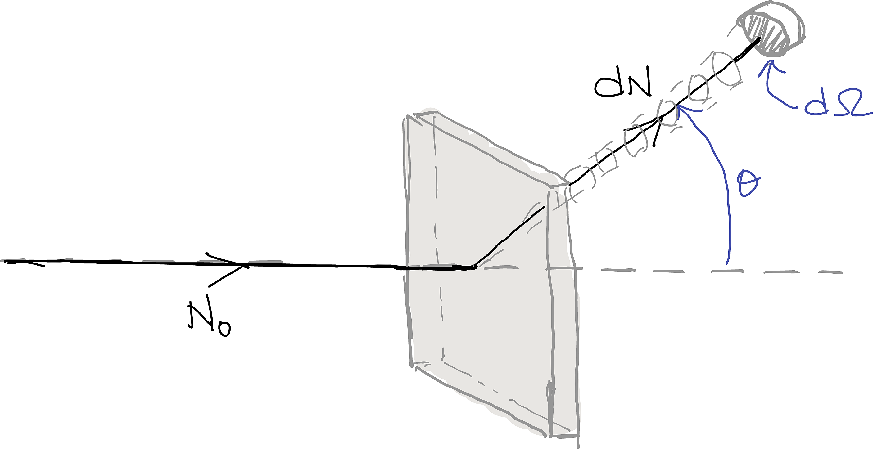
\[ dN = N_0nl \left(\frac{d\sigma}{d\Omega}\right)d\Omega. \tag{9.17}\]
The angular differential cross-section
\[ \frac{d\sigma}{d\Omega} \tag{9.18}\]
has units of area per steradian, such as \(\mathrm{b\,sr^{-1}}\). Integrating over all directions gives
\[ \sigma = \int_{4\pi} \frac{d\sigma}{d\Omega}\,d\Omega. \tag{9.19}\]
We can also construct doubly differential cross-sections to obtain even more detailed information. For example,
\[ dN = N_0nl \lr{\frac{\partial^2\sigma} {\partial\theta\,\partial\phi}} \,d\theta\,d\phi \tag{9.20}\]
gives the number of events scattered into the intervals \(\theta\) to \(\theta+d\theta\) and \(\phi\) to \(\phi+d\phi\).
Another commonly encountered example is
\[ \frac{d^2\sigma}{dE\,d\Omega}, \]
which describes how the outgoing particles are distributed in both energy and direction.
9.7 Some Types of Cross-Sections
| Type of Cross Section | Symbol | Related to | Possible Applications |
|---|---|---|---|
| Total | \(\sigma_t\) | Probability of any scattering event. | Shielding |
| Reaction | \(\sigma\) | Probability of any scattering event. | Production of radioisotope \(Y\) in nuclear reaction |
| Differential (Angular) | \(\frac{d\sigma}{d\Omega}\) | Probability of a scattering event that results in particles going into the solid angle \(d\Omega\) | Formation of a beam of particles in a certain direction (or recoil of \(Y\) in a certain direction) |
| Differential (Energy) | \(\frac{d\sigma}{dE}\) | Probability of a scattering event that results in particles losing energy by an amount \(dE\) | Study of decay of excited states of \(Y\) by subsequent \(\gamma\) emission of \(Y\) |
| Doubly differential (Energy & Angular) | \(\frac{\partial^2\sigma}{\partial E_{\beta}\partial\Omega}\) | Probability of a scattering event that results in particles going into the solid angle \(d\Omega\) and losing an amount of energy \(dE\) | Information on excited states of \(Y\) by angular distribution of emitted particles. |
9.8 Impact Parameter
9.8.1 What is the impact parameter?
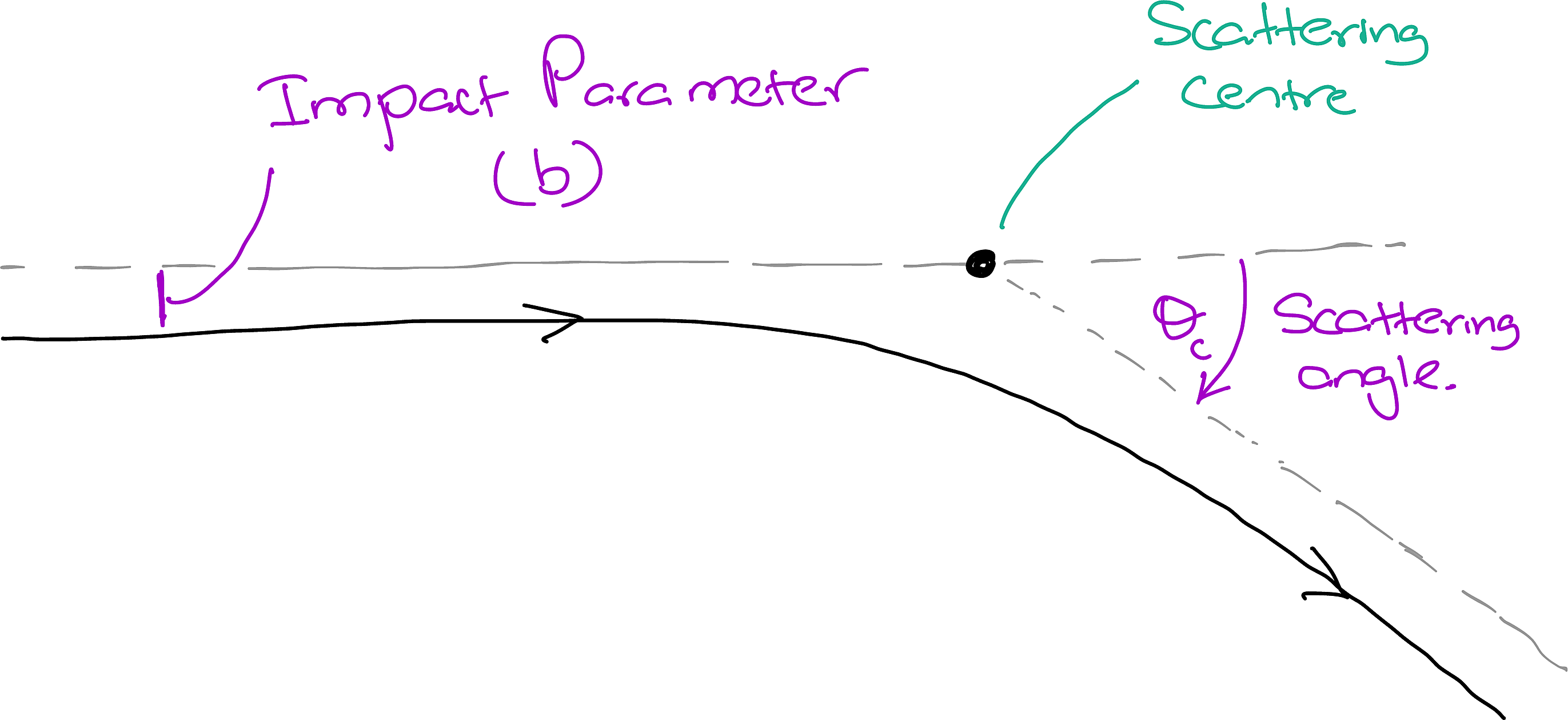
Consider a classical scattering event in which one particle interacts with another. The details of the scattering (such as whether the interaction is attractive or repulsive) depend on the interaction potential between the two particles. A useful quantity for describing such an event is the impact parameter (\(b\)). The impact parameter \(b\) is the perpendicular distance between the centre of the target and the projectile’s initial undeflected line of motion.
The usefulness \(b\) stems from the relationship between the impact parameter and the scattering angle, \(b=b(\theta)\). This relationship contains information about the interaction dynamics. It can be obtained by solving the classical scattering integral1,and 2.
For example, consider repulsive Coulomb scattering between two particles with charges \(ze\) and \(Ze\). This process is known as Rutherford scattering. In this case, a smaller impact parameter produces a larger scattering angle, and
\[ b = \frac{zZe^2}{4\pi\epsilon_0} \frac{1}{2E^*} \cot\left(\frac{\theta^*}{2}\right). \tag{9.21}\]
where \(E^*\) is the kinetic energy of the relative motion in the CM frame and \(\theta^*\) is the CM scattering angle.
9.8.2 How Is \(b\) Related to the total cross-section?
Consider an interaction that is azimuthally/cyclindrically symmetric about the incident-beam direction. Trajectories with impact parameters between \(b\) and \(b+db\) occupy a thin annulus of area \(2\pi b\,db\). But, recall that we interpreted a cross-section as an effective area representing the initial trajectories that produce a specified outcome. A cross-section is therefore built up from the contributions of many different impact parameters, with each annulus in the impact-parameter plane contributing to the cross-section for that outcome.
Hence,
\[ { d\sigma=2\pi b\,db }, \tag{9.22}\]
and
\[ { \sigma = 2\pi\int_0^{b_{max}} \,b\,db = \pi b_{max}^2 }. \tag{9.23}\]
Where, I have taken that all impact parameters below \(b_{max}\) contributes to the outcome we are interested in.
However, not all impact parameters necessarily contribute equally.
Let \(P(b)\) be the probability that a trajectory with impact parameter \(b\) produces the specified outcome. The contribution from the annulus is then
\[ { d\sigma=P(b)\,2\pi b\,db }. \tag{9.24}\]
The function \(P(b)\) is sometimes called the opacity function. Integrating over all possible impact parameters gives
\[ { \sigma = 2\pi\int_0^\infty P(b)\,b\,db }. \tag{9.25}\]
In effect, the interaction potential determines how a trajectory with a given impact parameter \(b\) evolves, while \(P(b)\) specifies the probability that the trajectory produces the particular outcome of interest. Adding the contributions from all impact parameters gives the cross-section for that outcome.
The form of \(P(b)\) can be complicated. In general, it may depend on the collision energy, the interaction potential and the selected reaction channel. As a simple approximation, however, consider a sharp cutoff:
\[ P(b)= \begin{cases} 1, & 0\leq b\leq b_{\max},\\ 0, & b>b_{\max}. \end{cases} \tag{9.26}\]
This approximation assumes that every trajectory with \(b\leq b_{\max}\) produces the specified outcome, while no trajectory with \(b>b_{\max}\) does. The total cross-section then becomes
\[ \sigma = 2\pi\int_0^{b_{\max}}b\,db = \pi b_{\max}^2. \tag{9.27}\]
So, the familiar geometrical relationship \({\sigma=\pi b_{\max}^2}\), is not a universal result. It is the sharp-cutoff limit of the more general impact-parameter expression Equation 9.25.
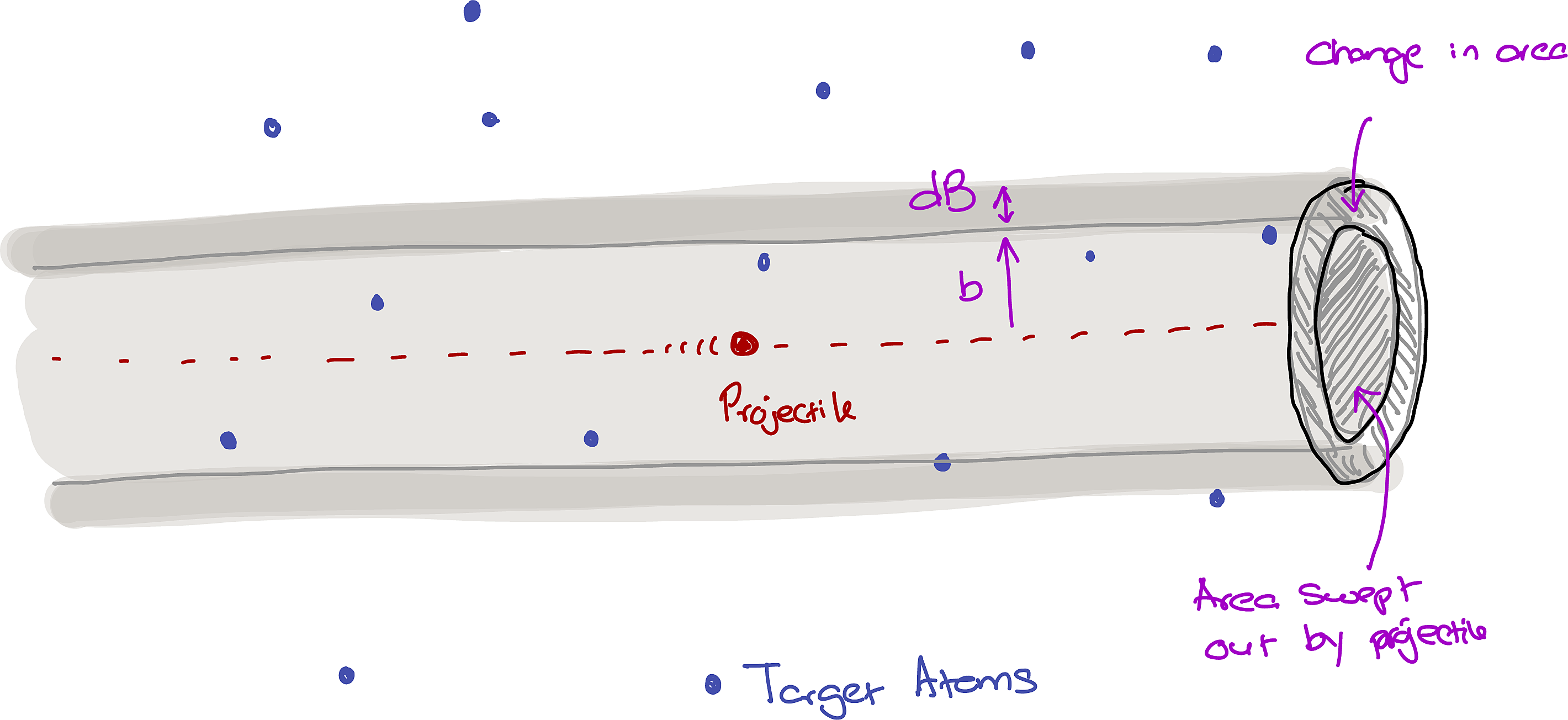
Assume that the incoming projectiles are distributed uniformly and that the interaction is azimuthally symmetric. In a plane perpendicular to the incident beam, projectiles with impact parameters between \(b\) and \(b+db\) occupy an annulus of area
\[ d\sigma=2\pi b\,db. \tag{9.28}\]
Therefore,
\[ \frac{d\sigma}{db}=2\pi b. \tag{9.29}\]
This is a geometrical result. The interaction physics enters through the relationship between the impact parameter and the scattering angle, \(b(\theta)\).
9.8.3 How Is \(b\) Related to the Differential Cross-Section?
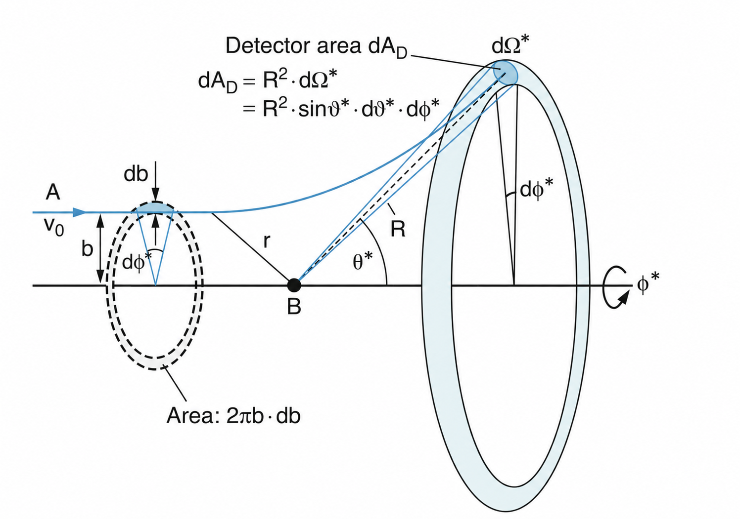
In experimental work, we often require more detailed predictions than a total cross-section can provide. We therefore need to connect the impact parameter \(b\) to the scattering angle \(\theta\) and, ultimately, to the differential cross-section. The importance of this connection will become clear a bit later when I bring these ideas together to derive the Rutherford scattering cross-section.
The CM frame is usually the most convenient frame for scattering problems. Therefore, the following discussion takes place in the CM frame.
For a central interaction, the scattering angle is decided by the impact parameter: \(\theta^*=\theta^*(b).\)
Suppose that trajectories with impact parameters between \(b\) and \(b+db\) are scattered into the angular interval between \(\theta^*\) and \(\theta^*+d\theta^*\) as seen in Figure 9.6. For repulsive Rutherford scattering, increasing \(b\) decreases the scattering angle, so
\[ \frac{db}{d\theta^*}<0. \]
The number of particles associated with both descriptions (\(\theta^*\) and \(b\)) must be the same. So, using Equation 9.14, we may write
\[ dN = N_0nl \left | {\left(\frac{d\sigma}{d\theta^*}\right) d\theta^*} \right | = N_0nl \left |\left(\frac{d\sigma}{db}\right) db\right |. \]
Giving us,
\[ \frac{d\sigma}{d\theta^*} = \frac{d\sigma}{db} \left| \frac{db}{d\theta^*} \right|. \tag{9.30}\]
For an azimuthally symmetric scattering process, discussed previously, Equation 9.29 gives:
\[ \frac{d\sigma}{db}=2\pi b. \]
Therefore,
\[ \frac{d\sigma}{d\theta^*} = 2\pi b \left| \frac{db}{d\theta^*} \right|. \tag{9.31}\]
The absolute value is required because a cross-section must be non-negative.
In an experiment, however, we are usually interested in the number of particles reaching a detector that subtends a small solid angle at a particular scattering angle. It is therefore more natural to express the result as a differential cross-section with respect to solid angle \(\Omega^*\). More specifically, we want,
\[ \frac{d\sigma}{d\Omega^*}. \]

The solid angle describes the cone-like range of directions accepted by the detector. For an area \(A\) on the surface of a sphere of radius \(R\), it is defined as
\[ \Omega=\frac{A}{R^2}. \]
Equivalently, a small area element \(dA\) subtends the solid angle
\[ d\Omega=\frac{dA}{R^2}. \]
To bring the solid angle into the picture, consider the azimuthally symmetric situation shown in Figure 9.6. The solid-angle element between \(\theta^*\) and \(\theta^*+d\theta^*\) corresponds to a thin ring on a sphere of radius \(R\). Therefore,
\[ \begin{aligned} d\Omega^* &= \frac{ \overbrace{2\pi R\sin\theta^*}^{\text{circumference of ring}} \; \overbrace{R\,d\theta^*}^{\text{width of ring}} }{R^2} \\ &= 2\pi\sin\theta^*\,d\theta^*. \end{aligned} \tag{9.32}\]
Combining this with Equation 9.31 yields the result we want:
\[ { \frac{d\sigma}{d\Omega^*} = \frac{b}{\sin\theta^*} \left| \frac{db}{d\theta^*} \right| }. \tag{9.33}\]
9.9 Differential Cross-Sections in the CM and LAB Frames
It is often easier to calculate a scattering distribution in the CM frame, while measurements are made in the LAB frame. However, angular cross-sections will differ because an angle in one frame is not necessarily the same in another. So, we need to see how to differential cross-sections transform between the LAB and CM frames?
We can connect these teo frames by noting that the total number of particles collected by a detector as viewd from eith frame must be the same.
\[ \frac{d\sigma}{d\Omega^*}\,d\Omega^* = \frac{d\sigma}{d\Omega} d\Omega. \tag{9.34}\]
Consequently,
\[ { \frac{d\sigma}{d\Omega} = \frac{d\sigma}{d\Omega^*} \left| \frac{d\Omega^*}{d\Omega} \right| }. \tag{9.35}\]
The factor relating the two differential cross-sections is a Jacobian that tells us how an angular interval in one frame maps a angular interval in the other.
For an azimuthally symmetric distribution,
\[ d\Omega^* = 2\pi\sin\theta^*\,d\theta^* = -2\pi\,d(\cos\theta^*), \]
and similarly in the LAB frame:
\[ d\Omega=-2\pi\,d(\cos\theta). \]
We can Brining all of these together to recast Equation 9.35 as \[ \frac{d\sigma}{d\Omega} = \frac{d\sigma}{d\Omega^*} \left| \frac{d(\cos\theta^*)}{d(\cos\theta)} \right|. \tag{9.36}\]
Finally, We know from our discussion of the CM frame in Chapter 8, that for For the non-relativistic elastic collision,
\[ \cos\theta = \frac{\cos\theta^*+\zeta} {\sqrt{1+2\zeta\cos\theta^*+\zeta^2}}, \qquad \zeta=\frac{m_1}{m_2}. \]
We can then reast Equation 9.36 wsing this relationshipto get:
\[ { \left(\frac{d\sigma}{d\Omega}\right)_{\mathrm{LAB}} = \frac{d\sigma}{d\Omega^*} \frac{ \left(1+2\zeta\cos\theta^*+\zeta^2\right)^{3/2} }{ \left|1+\zeta\cos\theta^*\right| } }. \tag{9.37}\]
9.10 Rutherford Scattering Cross-Section

The most convincing evidence for the existence of a small, dense atomic nucleus came from the gold-foil experiments conducted by Geiger and Marsden and interpreted by Rutherford3. The experiment is shown schematically in Figure 9.8.
Let us now bring together the ideas developed in the preceding sections to derive the famous Rutherford scattering cross-section.
For repulsive Coulomb scattering between particles with charges \(ze\) and \(Ze\), the classical relationship between the impact parameter and the CM scattering angle is
\[ b = \frac{zZe^2}{4\pi\epsilon_0} \frac{1}{2E^*} \cot\left(\frac{\theta^*}{2}\right), \tag{9.38}\]
where \(E^*\) is the kinetic energy associated with the relative motion in the CM frame.
To simplify the derivation, define
\[ a \equiv \frac{zZe^2}{4\pi\epsilon_0} \frac{1}{2E^*}. \]
Then,
\[ b=a\cot\left(\frac{\theta^*}{2}\right), \tag{9.39}\]
and hence
\[ \frac{db}{d\theta^*} = -\frac{a}{2} \csc^2\left(\frac{\theta^*}{2}\right). \]
Recall from Equation 9.33 that
\[ \left(\frac{d\sigma}{d\Omega}\right)^* = \frac{b}{\sin\theta^*} \left| \frac{db}{d\theta^*} \right|. \]
Substituting the expressions for \(b\) and \(db/d\theta^*\) gives
\[ \left(\frac{d\sigma}{d\Omega}\right)^* = \frac{ a\cot(\theta^*/2) }{ \sin\theta^* } \frac{a}{2} \csc^2\left(\frac{\theta^*}{2}\right). \]
Using
\[ \sin\theta^* = 2\sin\left(\frac{\theta^*}{2}\right) \cos\left(\frac{\theta^*}{2}\right), \]
we obtain
\[ \left(\frac{d\sigma}{d\Omega}\right)^* = \frac{a^2}{4} \frac{1}{\sin^4(\theta^*/2)}. \]
Replacing \(a\) with the original variables gives the Rutherford scattering formula:
\[ { \left(\frac{d\sigma}{d\Omega}\right)^* = \left( \frac{zZe^2}{16\pi\epsilon_0E^*} \right)^2 \frac{1}{\sin^4(\theta^*/2)} }. \tag{9.40}\]
The \(\sin^{-4}(\theta^*/2)\) dependence tells us that small-angle scattering is far more common than large-angle scattering. Nevertheless, the observation of even a small number of particles scattered through large angles—and, in some cases, almost directly backwards—provided the crucial evidence that the positive charge and most of the mass of an atom are concentrated within a very small nucleus.
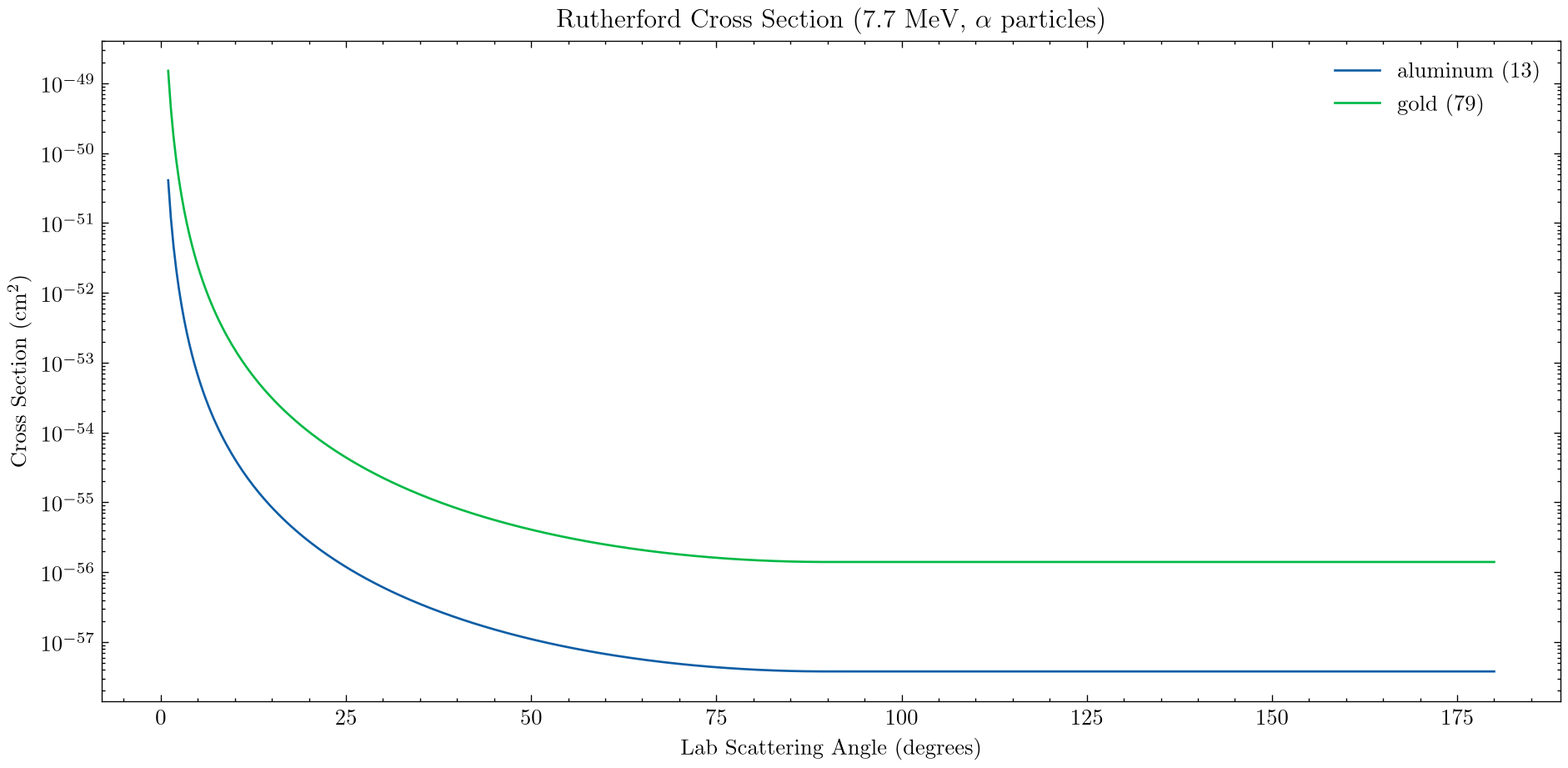
9.10.1 Why the Ideal Total Cross-Section Diverges
The ideal Rutherford differential cross-section diverges as $ ^*.$ Leading to the total cross-section,
\[ \sigma_{\mathrm{tot}} = \int_{4\pi} \left(\frac{d\sigma}{d\Omega}\right)^* d\Omega^*, \tag{9.41}\]
not to converge.
This happens because the ideal Rutherford model uses an unscreened Coulomb interaction with infinite range. Real experiments do not observe this divergence without limit. Atomic-electron screening weakens the Coulomb field at large distances. So, more realsitc cross-sections employ a screening length; which is a topic a fiels of its own.
9.11 Mean Free Path (\(\lambda\))
9.11.1 Free-Flight Distance
The picture developed so far is that particles travel through a material and interact with its scattering centres. The probability of an interaction depends on the number density \(n\) of the centres and the cross-section \(\sigma\) for the specified process.
From this perspective, we can ask: How far will a particle travel before undergoing an interaction? The answer leads us to the useful concept of the mean free path.
Let \(Q(x)\) be the probability that a particle travels a distance \(x\) without undergoing the specified interaction. We expect this probability to decrease as \(x\) increases:
\[ Q(x_{\mathrm{large}})<Q(x_{\mathrm{small}}). \]
Now consider the probability that the particle survives without interacting over a distance \(x+dx\). The particle must first travel the distance \(x\) without interacting and then survive the additional distance \(dx\). Therefore,
\[ Q(x+dx)=Q(x)Q(dx). \]
For a sufficiently small distance \(dx\), the probability of an interaction is
\[ n\sigma\,dx. \]
Therefore, the probability of passing through this distance without interacting is
\[ Q(dx)=1-n\sigma\,dx. \]
It follows that
\[ Q(x+dx) = Q(x)\left(1-n\sigma\,dx\right). \]
The change in the survival probability is
\[ \begin{aligned} dQ &= Q(x+dx)-Q(x) \\ &= Q(x)\left(1-n\sigma\,dx\right)-Q(x) \\ &= -n\sigma Q(x)\,dx. \end{aligned} \]
Therefore,
\[ \frac{dQ}{dx}=-n\sigma Q. \tag{9.42}\]
Separating the variables gives
\[ \frac{dQ}{Q}=-n\sigma\,dx. \]
Using the initial condition
\[ Q(0)=1, \]
we obtain
\[ { Q(x)=e^{-n\sigma x} }. \tag{9.43}\]
This is the probability that a particle travels at least a distance \(x\) without undergoing the specified interaction.
We now define the mean free path as
\[ { \lambda=\frac{1}{n\sigma} }. \tag{9.44}\]
The survival probability can therefore be written as
\[ { Q(x)=e^{-x/\lambda} }. \tag{9.45}\]
The mean free path is the characteristic distance over which the number of particles that have not interacted falls by a factor of \(e\):
\[ Q(\lambda)=e^{-1}. \]
Notice that the mean free path becomes shorter when either the number density \(n\) or the cross-section \(\sigma\) increases. A material containing more interaction centres or an interaction with a larger cross-section gives a particle fewer opportunities to travel freely.
9.11.2 Mean Free Path
Now we can answer the question ‘what is the mean distance traveled by a particle before an interaction?’.
Let’s say that a particle travels a distance \(x\) and then suffers a collision in the next \(dx\). The probability of this is given by: \(Q(x) \times n\sigma\,dx\).
We can use this to get at the mean value of \(x\) by:
\[ \exp{x} = \int_{x=0}^{x=\infty} x (e^{-x/\lambda} n\sigma dx) = \lambda \]
If the scattering centres have molar mass \(M\) and the material has mass density \(\rho\), then
\[ n=\frac{\rho N_A}{M}, \]
where \(N_A\) is Avogadro’s constant. Hence,
\[ { \lambda = \frac{1}{n\sigma} = \frac{M}{N_A\rho\sigma} }. \tag{9.46}\]