16 Nuclear reactions
\[ \newcommand\v[1]{\boldsymbol{#1}} \newcommand\vdot[2]{\v{#1}\cdot\v{#2}} \]
\[ \newcommand{\dd}[2][]{\mathrm{d}^{#1}#2} \]
\[ \newcommand\f[2]{\dfrac{#1}{#2}} \newcommand\da[2]{\dfrac{d #1}{d #2}} \newcommand\daa[2]{\dfrac{d^2 #1}{d #2^2}} \newcommand\pa[2]{\dfrac{\partial #1}{\partial #2}} \newcommand\pal[3]{\left.\dfrac{\partial #1}{\partial #2}\right|_{#3}} \newcommand\paa[2]{\dfrac{\partial^2 #1}{\partial #2^2}} \newcommand\pab[3]{\dfrac{\partial^2 #1}{\partial #2 \partial #3}} \def\half{\frac{1}{2}} \]
\[ \newcommand\ket[1]{\left|#1\right\rangle} % |x> \newcommand\exp[1]{\left\langle#1\right\rangle} % <x> \newcommand\lr[1]{\left(#1\right)} % (x) \newcommand\lrs[1]{\left[#1\right]} % [x] \newcommand\lra[1]{\left|#1\right|} % |x| \newcommand\lrc[1]{\left\{#1\right\}} % {x} \newcommand\lrl[3]{\left.#1\right|_{#2}^{#3}} % x_limits \]
\[ \def\ie{\text{i.e.}\quad} \]
\[ \newcommand{\me}[3][\rightarrow]{{#2}#1{#3}} % Typical reaction \newcommand{\nr}[3]{{#1}\,({#2})\,{#3}} % Nuclear reactions \newcommand{\ele}[4]{_{#2}^{#3}{\textbf{#1}}_{#4}} \newcommand{\el}[2]{^{#2}\text{#1}} \newcommand{\til}[2][\mathbf{\sim}]{\underset{#1}{{#2}}} \newcommand{\b}[1]{\overline{#1}} \]
\[ \newcommand{\coulomb}[1]{\dfrac{#1}{4\pi\epsilon_0}} \def\degree{^*} \]
\[ \def\amu{\text{ amu}} \def\J{\text{ J}} \def\K{\text{ K}} \def\s{\text{ s}} \def\second{\text{ s}} \def\Psecond{\text{ s}^{-1}} \def\m{\text{ m}} \def\mm{\text{ mm}} \def\km{\text{ km}} \def\fm{\text{ fm}} \def\mum{\text{ $\mu$m}} \def\mus{\text{ $\mu$s}} \def\mPERs{\text{ ms$^{-1}$}} \def\eV{\text{ eV}} \def\keV{\text{ keV}} \def\GeV{\text{ GeV}} \def\MeV{\text{ MeV}} \def\MeVc{\text{ MeV/c$^2$}} \def\KeVc{\text{ KeV/c$^2$}} \newcommand\ttp[1]{\times 10^{#1}} % To The Power \]
\[ \def\en{\nu_e} \def\Aen{\b{\nu_e}} \def\mun{\nu_\mu} \def\Amun{\b{\nu}_\mu} \]
\[ \def\uraniumA{\ele{U}{92}{233}{}} \def\uraniumB{\ele{U}{92}{235}{}} \def\uraniumC{\ele{U}{92}{238}{}} \def\carbonB{\ele{C}{6}{14}{}} \def\nitrogenB{\ele{N}{7}{14}{}} \def\oxygenA{\ele{O}{8}{14}{}} \def\oxygenB{\ele{O}{8}{16}{}} \]
\[ % \def\com{\text{\scriptsize CM}} \def\com{\mathrm{\scriptsize CM}} \]
\[ \def\l{l} \]
\[ \def\g{\gamma} \]
What To Expect In This Chapter
Most of our knowledge about nuclei and particle physics comes from shooting particles at other particles. We discussed some aspects of this when introducing cross-sections. In this chapter, I will focus on a particular subset of reactions involving nuclei.
For example, in 1919, Rutherford observed that some \(\alpha\) particles passing through a sample of nitrogen participated in the following transmutation reaction:
\[ \me{\alpha+\ele{N}{7}{14}{}}{\ele{O}{8}{17}{}+p}. \tag{16.1}\]
These reactions are fundamentally different from ordinary scattering because the projectile has sufficient energy to penetrate the Coulomb barrier, get close enough to the target nucleus, and initiate a nuclear reaction.
Many nuclear technologies, including nuclear energy, neutron scattering, and some forms of radiation therapy, involve nuclear reactions. Understanding their basic properties is therefore important.
16.1 Types of Reactions, Observables, and Conserved Quantities
16.1.1 Types of Reactions
Here are a few examples of nuclear reactions:
\[ \begin{align} \me[&\rightarrow]{\alpha+\ele{N}{7}{14}{}}{\ele{O}{8}{17}{}+p} &&\color{gray}{\nr{\ele{N}{7}{14}{}}{\alpha,p}{\ele{O}{8}{17}{}}}\\[1em] \me[&\rightarrow]{p+\ele{Li}{3}{7}{}}{\ele{He}{2}{4}{}+\alpha} &&\color{gray}{\nr{\ele{Li}{3}{7}{}}{p,\alpha}{\ele{He}{2}{4}{}}}\\[1em] \me[&\rightarrow]{p+\ele{Na}{11}{23}{}}{\ele{Na}{11}{22}{}+n+p} &&\color{gray}{\nr{\ele{Na}{11}{23}{}}{p,np}{\ele{Na}{11}{22}{}}}\\[1em] \me[&\rightarrow]{\alpha+\alpha+\alpha}{\ele{C}{6}{12}{}} \end{align} \tag{16.2}\]
I have indicated an alternative, convenient notation on the right. A typical nuclear reaction can be written as
\[ \me{a+X}{Y+b}, \tag{16.3}\]
where \(a\) is the projectile, \(X\) is the target, and \(Y\) and \(b\) are the products.
Usually, \(Y\) is the heavy recoil nucleus and typically stop inside the target. It is often the lighter product \(b\), such as a proton, neutron, \(\alpha\) particle, or \(\gamma\) ray, that escapes and is detected.
We usually abbreviate Equation 16.3 as
\[ \nr{X}{a,b}{Y}. \tag{16.4}\]
This notation is useful because it categorises reactions by their incoming projectile and observed outgoing particle. Examples include \((\alpha,n)\), \((n,p)\), and \((n,\gamma)\) reactions.
The following table summarises common types of nuclear reactions.
| Type of reaction | General characteristics | Additional details |
|---|---|---|
| Scattering | \(X=Y\) | - Elastic: \(Y\) and \(b\) are in their ground states. - Inelastic: \(Y\) or/and \(b\) are in an excited state. |
| Knockout | \(b = a\), but other additional particle(s) gets ejected. | |
| Direct | Only a few nucleons of \(X\) and \(b\) take part in the reaction. The remaining nucleons of the target serve as spectators. | - Transfer reactions: One or two nucleons are transferred between the projectile and target |
| Compound nucleus | \(a\) and \(X\) merge briefly for a complete sharing of energy before the outgoing nuclei is ejected | |
| Resonance | \(a\) and \(X\) form a ‘quasi bound’ state before the outgoing particle is ejected. | This category lies between direct and compound nucleus reactions. |
| Type of reaction | General characteristics | Additional details |
|---|---|---|
| Scattering | The projectile and target remain the same species: \(a=b\) and \(X=Y\). | - Elastic scattering: both outgoing particles remain in their ground states. - Inelastic scattering: the projectile or target is left in an excited state. |
| Knockout | The incident projectile emerges as the same particle, \(b=a\), while one or more nucleons are ejected from the target. | Examples include \((p,2p)\) and \((p,pn)\) reactions. |
| Direct | Only a few nucleons of the projectile \(a\) and target \(X\) take part directly in the reaction. The remaining target nucleons act mainly as spectators. | - Transfer reactions: one or more nucleons are transferred between the projectile and target. |
| Compound nucleus | The projectile \(a\) and target \(X\) merge briefly to form a compound nucleus. Its energy is shared among many nucleons before it decays into outgoing products. | The decay products need not retain a strong memory of the initial projectile direction. |
| Resonance | The projectile and target form a short-lived quasi-bound state at a particular incident energy before decaying. | Resonances appear as peaks in reaction cross-sections. They are often associated with compound-nucleus states. |
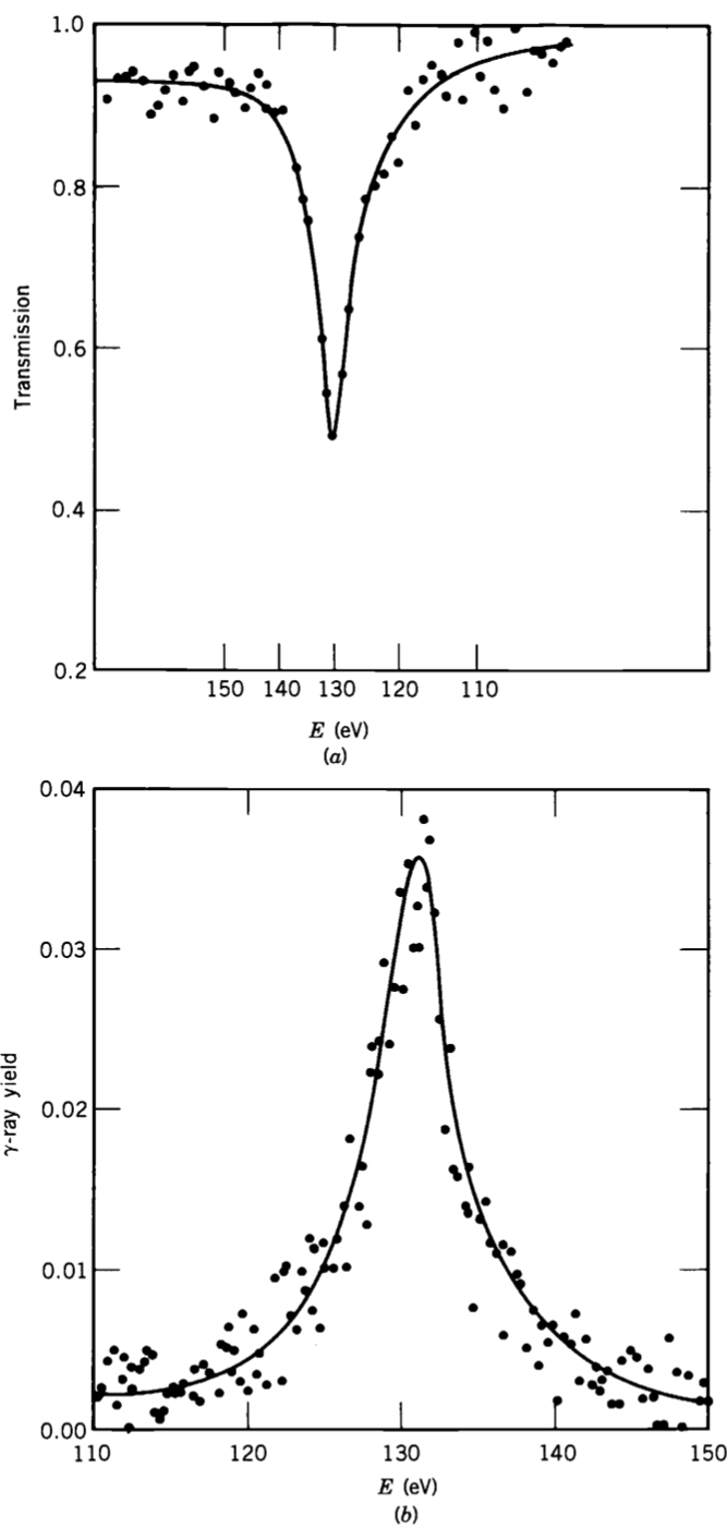
Recall that we encountered the idea of resonances when discussing particle physics. You can think of a resonance as a “bump” in a reaction cross-section. This means that the particles interact or react more strongly at particular projectile energies.
This heightened interaction occurs when the energy of the incoming projectile and target corresponds to an excited state of the combined, or compound, system \(a+X\).
Figure Figure 16.1 illustrates this idea for neutron interactions with \({}^{59}\mathrm{Co}\). Figure (a) shows the intensity of neutrons transmitted through the cobalt target. At a resonance, the reaction probability is high, so the intensity of the transmitted neutron beam drops to a minimum.
Figure (b) shows the \(\gamma\)-ray yield from neutron radiative capture by \({}^{59}\mathrm{Co}\). Here, the \(\gamma\)-ray yield is largest where the reaction probability is largest.
16.1.2 Observables
The resonance figure gives us a useful introduction to the quantities measured in nuclear-reaction experiments.
Typical experimental setups allow us to measure:
- the identity of the outgoing particles;
- the energy of outgoing particles, often to a resolution of several \(\mathrm{keV}\);
- the reaction yield or cross-section, which tells us how likely a particular reaction is to occur;
- the angular distribution of outgoing particles, by placing detectors at different angles \((\theta,\phi)\) relative to the original beam direction;
- the polarization of outgoing particles;
- coincidences, where two or more correlated outgoing particles or \(\gamma\) rays are detected together.
For photons, polarization refers to classical linear polarization. For particles such as protons and neutrons, it refers to the direction of their spin, measured using an appropriate spin-sensitive apparatus.
Polarization measurements are useful because they reveal how a reaction depends on spin orientation. They can help us determine the spin and parity of nuclear states, identify the angular momenta involved in a reaction, and distinguish between possible reaction mechanisms.
16.1.3 Conserved Quantities
Let us now consider what is, and is not, conserved during a nuclear reaction.
Energy, momentum, electric charge, and baryon number are always conserved. These conservation laws are very useful for extracting details of a reaction, such as the excitation energy of a final nucleus.
Most reactions discussed in this chapter are driven by the strong or electromagnetic interactions. These interactions conserve parity. Weak nuclear processes, such as \(\beta\) decay, do not conserve parity, but they usually occur on much longer timescales and will not be our focus here.
16.2 \(Q\) Value
\[ \newcommand\t[1]{(m_{#1}c^2+T_{#1})} \]
Let me now introduce a quantity you will encounter often in nuclear reactions and decays. It is called the \(Q\) value, and it tells us the net energy released in a reaction or decay:
\[ Q = \left[ m_{\text{initial}}-m_{\text{final}} \right]c^2. \tag{16.5}\]
For a reaction of the type
\[ \nr{X}{a,b}{Y} \qquad\text{or}\qquad \me{a+X}{Y+b}, \]
we have
\[ Q = \left[ (m_a+m_X)-(m_Y+m_b) \right]c^2. \tag{16.6}\]
Using conservation of total energy gives
\[ m_ac^2+T_a+m_Xc^2+T_X = m_Yc^2+T_Y+m_bc^2+T_b. \]
Rearranging, we obtain
\[ Q = (T_Y+T_b)-(T_a+T_X). \tag{16.7}\]
Thus, the \(Q\) value is the difference between the final and initial total kinetic energies:
\[ Q = T_{\text{final}}-T_{\text{initial}}. \tag{16.8}\]
- \(Q>0\) describes an exothermic reaction. Mass energy or binding energy has been converted into kinetic energy.
- \(Q<0\) describes an endothermic reaction. Kinetic energy must be supplied to make the reaction possible.
16.2.1 \(Q\) Value and Excited States
One or more final nuclei may be produced in an excited state. In this case, some of the available energy goes into excitation rather than kinetic energy.
If the final products \(i\) have excitation energies \(E_i^*\), then
\[ Q = Q_0-\sum_i E_i^*, \tag{16.9}\]
where \(Q_0\) is the \(Q\) value for the reaction in which all products are in their ground states.
16.3 General Properties
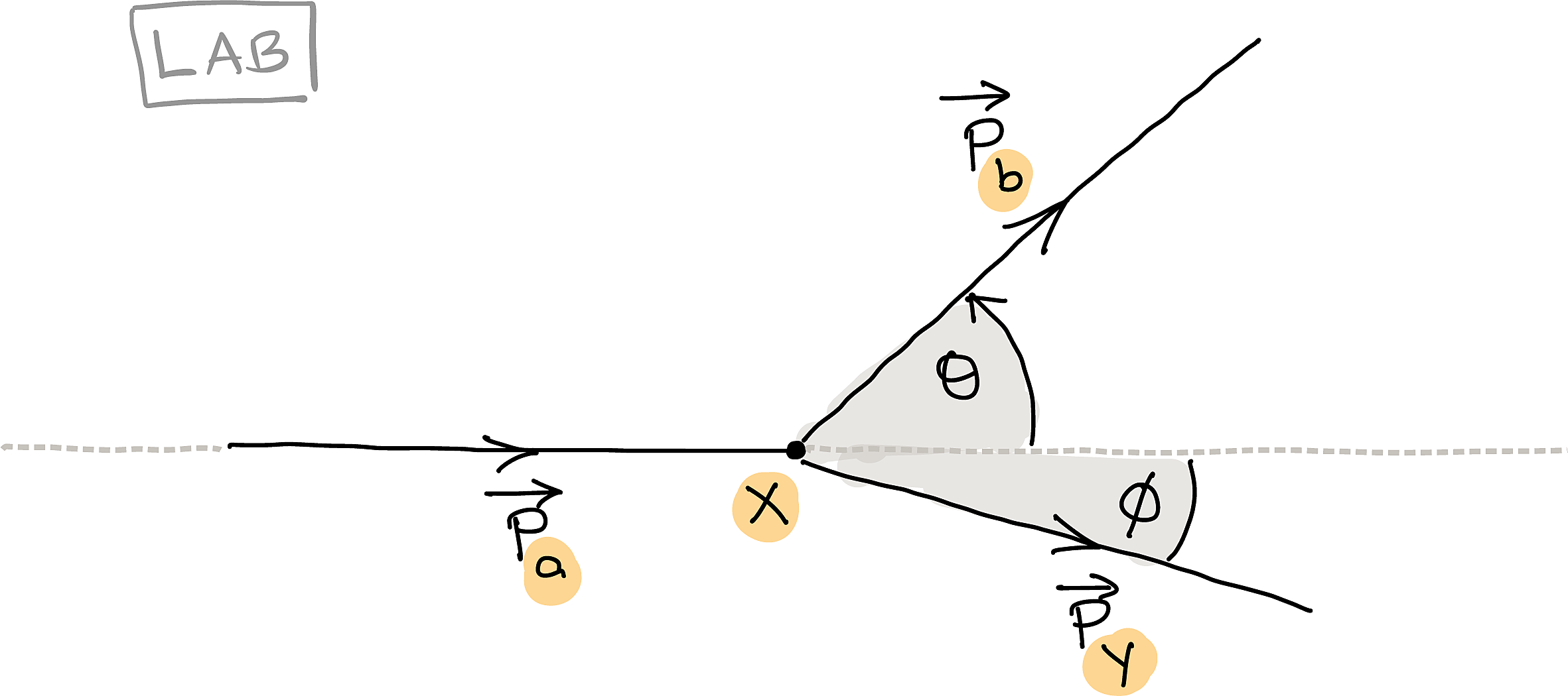
Let us use conservation laws to identify some general properties of a reaction of the type \(\nr{X}{a,b}{Y}\), shown in Figure 16.2.
Notice that the particles emerging from the reaction are different from those entering it. We will work in the LAB frame, where the target \(X\) is initially at rest.
If you are worried about thermal motion, note that at room temperature,
\[ k_BT\approx10^{-2}\,\mathrm{eV}, \]
which is negligible compared with the \(\mathrm{keV}\) or \(\mathrm{MeV}\) energies of most nuclear-reaction experiments.
Energy and momentum conservation give
\[ \begin{aligned} Q &= (T_Y+T_b)-(T_X+T_a),\\ p_a &= p_b\cos\theta+p_Y\cos\phi,\\ 0 &= p_b\sin\theta-p_Y\sin\phi. \end{aligned} \tag{16.10}\]
The heavy recoil nucleus \(Y\) is often difficult to detect directly. However, by measuring the incident particle \(a\) and the outgoing particle \(b\), we can still learn a great deal about the reaction.
In an experiment, we control the incident momentum \(\v{p}_a\), and hence the incident kinetic energy \(T_a\). Let us assume that \(Q\) is known and determine the possible values of the kinetic energy \(T_b\) of the outgoing particle.
Since nuclear masses are typically of the order of \(10^3\,\mathrm{MeV}/c^2\), and many nuclear reactions involve kinetic energies of a few \(\mathrm{MeV}\), the particles involved are often non-relativistic. For such particles,
\[ T=\f{p^2}{2m}. \]
Using this relation to eliminate \(\phi\) and the momenta in Equation 16.10 gives a quadratic equation for \(T_b^{1/2}\). Its solutions are
\[ T_b^{1/2} = \f{ \left(m_am_bT_a\right)^{1/2}\cos\theta \pm \left\{ m_am_bT_a\cos^2\theta + \left(m_Y+m_b\right) \left[ m_YQ+\left(m_Y-m_a\right)T_a \right] \right\}^{1/2} }{ m_Y+m_b }. \tag{16.11}\]
We can learn a great deal about nuclear reactions from this relationship.
16.3.1 For \(Q<0\), There Is an Absolute Minimum Value of \(T_a\)
For a reaction to occur, the quantity inside the square root in Equation 16.11 must be non-negative:
\[ \begin{align} m_am_bT_a&\cos^2\theta + \left(m_Y+m_b\right) \left[ m_YQ+\left(m_Y-m_a\right)T_a \right] \geq0.\\ \Rightarrow T_a& \lr{m_{a}m_{b}\cos ^{2}\theta + ( m_y+m_{b})( m_y-m_{a}) } \geq (-Q)\,m_y(m_y+m_b) \\ \ie T_a& \geq (-Q)\lrs{\f{m_y(m_y+m_b)}{m_{a}m_{b}(\cos ^{2}\theta-1) + m_y(m_b-m_a) + m^2_y }} \end{align} \tag{16.12}\]
For \(Q<0\), the incident particle must supply a minimum amount of kinetic energy. The absolute threshold energy is found by considering the most favourable case, \(\theta=0\):
\[ T_{\text{th}} = -Q \lrs{ \f{m_Y+m_b}{m_Y+m_b-m_a} }. \tag{16.13}\]
Below \(T_{\text{th}}\), no reaction can occur.
For \(Q>0\), there is no kinematic threshold energy of this type. However, a charged projectile must still have sufficient energy to penetrate the Coulomb barrier and reach the target nucleus.
16.3.2 A Double-Valued Situation Can Occur for \(Q<0\)
The \(\pm\) sign in Equation 16.11 indicates that two values of \(T_b\) may be possible for the same incident energy and observation angle.
The \(+\)’ve solution is always permitted whenever the expression under the square root is non-negative. The \(-\)’ve solution is more restricted. In particular, it requires
\[ \begin{align} &\left( m_{a}m_{b}T_{a}\right)^{1/2}\cos \theta {\color{Maroon}{-}} \left\{ m_{a}m_{b}T_{a}\cos ^{2}\theta +\left( my+m_{b}\right)\left[m_{Y}Q+\left( m_{Y}-m_{a}\right) T_{a}\right]\right\}^{1/2} \geq 0\\ \Rightarrow &m_{a}m_{b}T_{a}\cos ^{2}\theta \geq m_{a}m_{b}T_{a}\cos ^{2}\theta +\left( my+m_{b}\right)\left[m_{Y}Q+\left( m_{Y}-m_{a}\right) T_{a}\right]\\ \Rightarrow &m_{Y}Q+\left( m_{Y}-m_{a}\right) T_{a} \leq 0 \\ \ie &T_a \leq {T}_a' \end{align} \tag{16.14}\]
Where I have used, \[ {T}_a' = -Q\lrs{\f{m_Y}{m_y-m_a}} \tag{16.15}\]
assuming a forward angle (\(\cos\theta\geq0\)) for the common case \(m_Y>m_a\).
Then the two solutions can occur when
\[ T_{\text{th}} \leq T_a \leq T_a'. \tag{16.16}\]
Thus, for an endothermic reaction, there can be two possible values of \(T_b\) for the same value of \(T_a\) and the same detector angle.
16.3.3 Not All Angles Are Allowed
Even when \(T_{\text{th}}\leq T_a\leq T_a'\), the expression under the square root in Equation 16.11 can become negative at sufficiently large angles. This is because \(Q<0\) already reduces the available kinetic energy, while \(\cos^2\theta\) decreases as the scattering angle increases.
From Equation 16.12, \[ \begin{align} m_{a}m_{b}T_{a}\cos ^{2}\theta +(m_{Y}+m_{b})\lrs{m_{Y}Q+(m_Y-m_a)T_a} \geq 0 \\ \Rightarrow \cos^2 \theta \geq -\f{(m_{Y}+m_{b})\lrs{m_{Y}Q+(m_Y-m_a)T_a}}{m_{a}m_{b}T_{a}} \end{align} \tag{16.17}\]
For the usual forward-angle range, this defines a maximum allowed angle, \(\theta_{\max}\) such that:
\[ \theta \leq \theta_{\max}. \tag{16.18}\]
where: \[ \cos^2\theta_{\max} = -\f{ (m_Y+m_b) \lrs{ m_YQ+\left(m_Y-m_a\right)T_a } }{ m_am_bT_a }. \tag{16.19}\]
For angles smaller than \(\theta_{\max}\), two outgoing energies may be possible. At \(\theta=\theta_{\max}\), the two solutions merge. For larger angles, there is no real kinematic solution.
16.3.4 A Concrete Example
The following interactive plot shows the possible values of \(T_b\) for the reaction
\[ \ele{H}{1}{3}{}(p,n)\ele{He}{2}{3}{}. \]
For this reaction,
\[ Q=-763.75\,\mathrm{keV}. \]
- The dashed lines represent \(T_{\text{th}}\) and \(T_a'\).
- Zoom into the lower-left region to see the two possible values of \(T_b\).
- For \(T_a>T_a'\), only one branch remains, so there is a one-to-one relationship between \(T_b\) and \(\theta\) for a fixed \(T_a\).
This also gives us a useful way to generate neutrons with a selected energy. At a fixed incident energy, a detector placed at a particular angle selects neutrons with a particular kinematically allowed energy. In the double-valued region, the two branches must be distinguished.
For \(T_a=1.1\,\mathrm{MeV}\), Equation 16.19 gives
\[ \theta_{\max}=54.83\degree. \]
The plots below show the behaviour at \(\theta_{\max}\) and at angles just below and above it.
At angles below \(\theta_{\max}\), two values of \(T_b\) are possible. At \(\theta_{\max}\), the two branches meet. At angles above \(\theta_{\max}\), the reaction is not kinematically allowed.
If we consider the reverse reaction,
\[ \ele{He}{2}{3}{}(n,p)\ele{H}{1}{3}{}, \]
then
\[ Q=+763.75\,\mathrm{keV}. \]
The dynamics now change drastically: the reaction is exothermic, and the double-valued region found above no longer occurs for this example.