7 About Parity
\[ \newcommand\v[1]{\boldsymbol{#1}} \newcommand\vdot[2]{\v{#1}\cdot\v{#2}} \]
\[ \newcommand{\dd}[2][]{\mathrm{d}^{#1}#2} \]
\[ \newcommand\f[2]{\dfrac{#1}{#2}} \newcommand\da[2]{\dfrac{d #1}{d #2}} \newcommand\daa[2]{\dfrac{d^2 #1}{d #2^2}} \newcommand\pa[2]{\dfrac{\partial #1}{\partial #2}} \newcommand\pal[3]{\left.\dfrac{\partial #1}{\partial #2}\right|_{#3}} \newcommand\paa[2]{\dfrac{\partial^2 #1}{\partial #2^2}} \newcommand\pab[3]{\dfrac{\partial^2 #1}{\partial #2 \partial #3}} \def\half{\frac{1}{2}} \]
\[ \newcommand\ket[1]{\left|#1\right\rangle} % |x> \newcommand\exp[1]{\left\langle#1\right\rangle} % <x> \newcommand\lr[1]{\left(#1\right)} % (x) \newcommand\lrs[1]{\left[#1\right]} % [x] \newcommand\lra[1]{\left|#1\right|} % |x| \newcommand\lrc[1]{\left\{#1\right\}} % {x} \newcommand\lrl[3]{\left.#1\right|_{#2}^{#3}} % x_limits \]
\[ \def\ie{\text{i.e.}\quad} \]
\[ \newcommand{\me}[3][\rightarrow]{{#2}#1{#3}} % Typical reaction \newcommand{\nr}[3]{{#1}\,({#2})\,{#3}} % Nuclear reactions \newcommand{\ele}[4]{_{#2}^{#3}{\textbf{#1}}_{#4}} \newcommand{\el}[2]{^{#2}\text{#1}} \newcommand{\til}[2][\mathbf{\sim}]{\underset{#1}{{#2}}} \newcommand{\b}[1]{\overline{#1}} \]
\[ \newcommand{\coulomb}[1]{\dfrac{#1}{4\pi\epsilon_0}} \def\degree{^*} \]
\[ \def\amu{\text{ amu}} \def\J{\text{ J}} \def\K{\text{ K}} \def\s{\text{ s}} \def\second{\text{ s}} \def\Psecond{\text{ s}^{-1}} \def\m{\text{ m}} \def\mm{\text{ mm}} \def\km{\text{ km}} \def\fm{\text{ fm}} \def\mum{\text{ $\mu$m}} \def\mus{\text{ $\mu$s}} \def\mPERs{\text{ ms$^{-1}$}} \def\eV{\text{ eV}} \def\keV{\text{ keV}} \def\GeV{\text{ GeV}} \def\MeV{\text{ MeV}} \def\MeVc{\text{ MeV/c$^2$}} \def\KeVc{\text{ KeV/c$^2$}} \newcommand\ttp[1]{\times 10^{#1}} % To The Power \]
\[ \def\en{\nu_e} \def\Aen{\b{\nu_e}} \def\mun{\nu_\mu} \def\Amun{\b{\nu}_\mu} \]
\[ \def\uraniumA{\ele{U}{92}{233}{}} \def\uraniumB{\ele{U}{92}{235}{}} \def\uraniumC{\ele{U}{92}{238}{}} \def\carbonB{\ele{C}{6}{14}{}} \def\nitrogenB{\ele{N}{7}{14}{}} \def\oxygenA{\ele{O}{8}{14}{}} \def\oxygenB{\ele{O}{8}{16}{}} \]
\[ % \def\com{\text{\scriptsize CM}} \def\com{\mathrm{\scriptsize CM}} \]
\[ \def\l{l} \]
\[ \def\g{\gamma} \]
What to Expect in This Chapter
In this chapter, I will discuss the fascinating idea of parity. At first sight, parity looks like a simple transformation of spatial coordinates. However, it also allows us to classify quantum states and to place useful restrictions on particle reactions and decays. Things become even more interesting when we discover that parity is conserved by the strong and electromagnetic interactions but violated by the weak interaction. We will finish by discussing the famous Wu experiment, which showed that nature can distinguish an experiment from its mirror image.
7.1 What Is Parity?
7.1.1 Parity Transformation \(\equiv\) Inversion
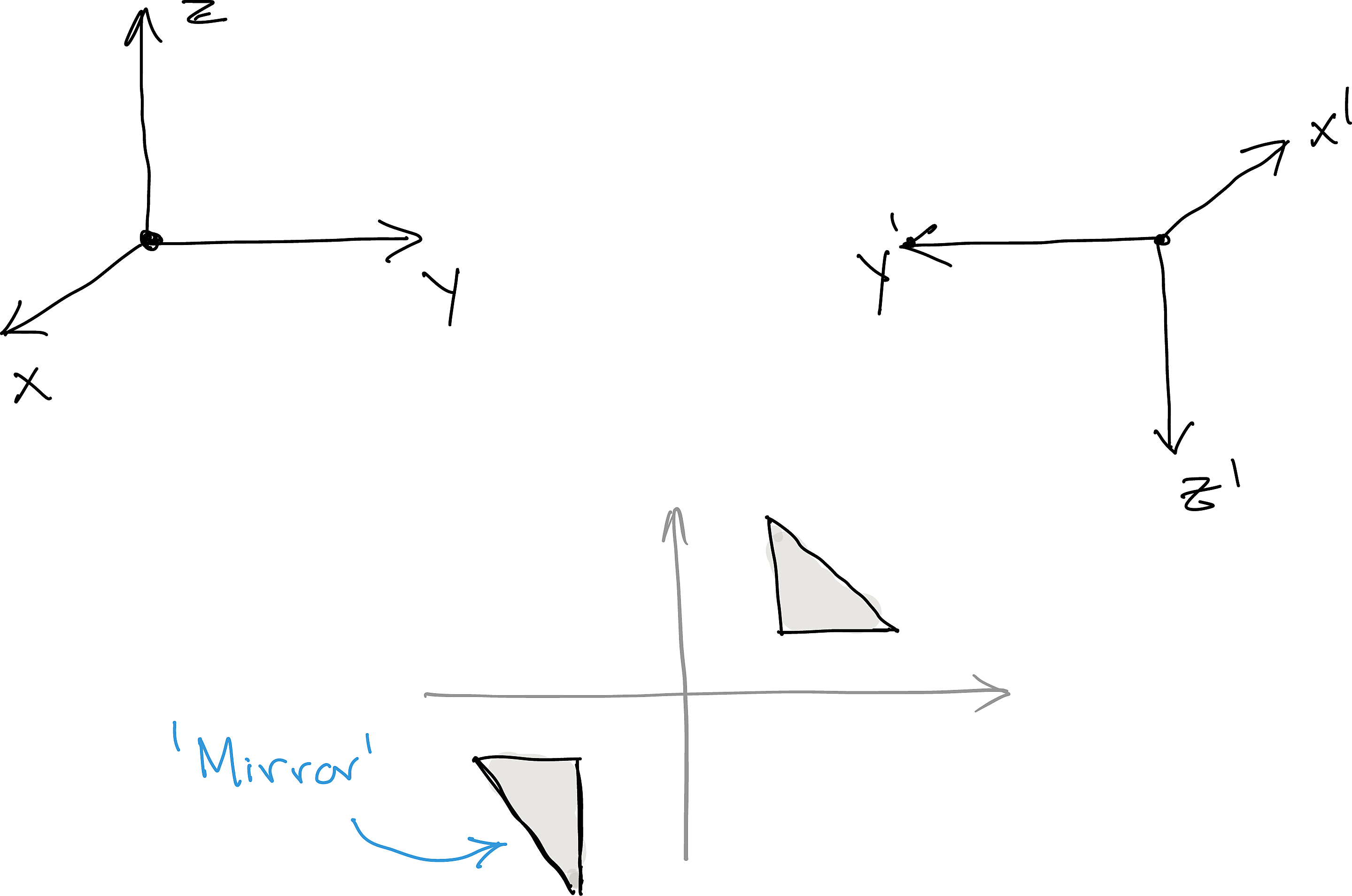
I have mentioned before that conservation laws are closely connected to symmetries in our universe. For example, translational symmetry (performing an experiment at \(x\) or at \(x+42\) should give the same result) leads through Noether’s theorem to the conservation of momentum. Physicists are therefore very interested in transformations and symmetries. An inversion, or parity transformation, reverses all three spatial coordinates: \[ \begin{array}{rcl} \text{General:} & \mathbf r &\longrightarrow -\mathbf r\\ \text{Cartesian:} & (x,y,z) &\longrightarrow (-x,-y,-z)\\ \text{Spherical:} & (r,\theta,\phi) &\longrightarrow (r,\pi-\theta,\phi+\pi) \end{array} \tag{7.1}\]
People often describe the parity-transformed arrangement as the “mirror universe”. However, inversion is not exactly the same as an ordinary reflection in a single mirror. A reflection in one plane must be followed by a rotation to reproduce a complete inversion.
To keep things simple, I will sometimes use real for the original arrangement and mirror for its parity-transformed counterpart. However, remember that these labels do not describe two physically separate universes; they describe two experimental arrangements that we want to compare.
7.1.2 Scalars, Vectors, Pseudoscalars and Pseudovectors
Parity gives us a more refined way of classifying physical quantities. In addition to the familiar distinction between scalars and vectors, we can identify pseudoscalars and pseudovectors.
| Type | Behaviour under parity | Typical examples |
|---|---|---|
| Scalar | Invariant | Mass, energy and electric charge |
| Pseudoscalar | \(Q\rightarrow-Q\) | \(\mathbf S\cdot\mathbf p\) |
| Polar vector | \(\mathbf V\rightarrow-\mathbf V\) | Position \(\mathbf r\), momentum \(\mathbf p\) and velocity \(\mathbf v\) |
| Axial vector or pseudovector | Invariant | Angular momentum \(\mathbf L\) and spin \(\mathbf S\) |
The quantity \(\mathbf S\cdot\mathbf p\) will become important when we discuss helicity later in the chapter.
7.1.3 Are We in the Real or the Mirror Universe?
Is there an experiment that can tell us whether we are looking at the original arrangement or its parity-transformed counterpart? Let us begin with Newton’s second law. Under parity, both force and acceleration reverse direction: \[ \mathbf F\longrightarrow-\mathbf F', \qquad \mathbf a\longrightarrow-\mathbf a'. \] Therefore, \[ \mathbf F=m\mathbf a \quad\longrightarrow\quad -\mathbf F'=m(-\mathbf a'). \tag{7.2}\] Newton’s law has exactly the same form after the transformation. We therefore cannot determine which arrangement is the “real” one by throwing a ball and watching its motion. What about angular momentum? \[ \mathbf L' = \mathbf r'\times\mathbf p' = (-\mathbf r)\times(-\mathbf p) = \mathbf L. \tag{7.3}\]
Angular momentum does not reverse under parity. The same is true of spin, \(\mathbf S\). Both are axial vectors. So far, the original and parity-transformed experiments are indistinguishable. The Wu experiment will eventually give us a way to tell them apart.
7.2 Quantum Mechanics of Parity
7.2.1 The Parity Operator
Let us introduce the parity operator, \(\hat P\). Acting on a wavefunction, it reverses the spatial coordinates:
\[ \hat P\psi(\mathbf r) = \psi(-\mathbf r). \tag{7.4}\]
Applying parity twice returns us to the original wavefunction:
\[ \hat P^2\psi(\mathbf r)=\psi(\mathbf r). \]
A state has definite parity if it is an eigenstate of \(\hat P\):
\[ \hat P\psi(\mathbf r) = \eta_P\psi(\mathbf r), \qquad \eta_P=\pm1. \tag{7.5}\]
Thus,
\[ \psi(-\mathbf r) = \begin{cases} +\psi(\mathbf r), & \eta_P=+1 \quad\text{(even parity)},\\[0.6em] -\psi(\mathbf r), & \eta_P=-1 \quad\text{(odd parity)}. \end{cases} \tag{7.6}\]
Important:
- Not every possible quantum state has definite parity1.
- Parity is not the same as the symmetric or antisymmetric exchange behaviour that appears in the spin–statistics theorem. Parity reverses spatial coordinates, whereas exchange symmetry describes what happens when two identical particles are interchanged. In some special situations these ideas may be related, but they are conceptually different.
7.2.2 Spatial and Intrinsic Parity
There are two contributions to parity that you need to recognise: intrinsic parity and relative spatial parity.
Consider the strong decay
\[ \me{\phi^0}{K^++K^-}. \tag{7.7}\]
Intrinsic parity: Each particle has an intrinsic parity associated with its internal quantum state. The \(\phi^0\), \(K^+\) and \(K^-\) therefore each carry intrinsic-parity factors.
Relative spatial parity: The two kaons can also carry orbital angular momentum because of their relative motion about their centre of mass. The angular part of this motion is described by a spherical harmonic, \(Y^\ell_m(\theta,\phi)\). Under parity,
\[ Y^\ell_m(\pi-\theta,\phi+\pi) = (-1)^\ell Y^\ell_m(\theta,\phi). \tag{7.8}\]
The relative spatial parity is therefore
\[ \eta_{\text{spatial}}=(-1)^\ell. \tag{7.9}\]
Parity is also important for composite nuclei. Their parity is commonly displayed together with their nuclear spin, as \(J^P\).
For example,
\[ 0^+ \quad\Rightarrow\quad J=0, \qquad P=+1. \]
If you are wondering where intrinsic parity and these particle–antiparticle rules come from, they ultimately arise from quantum field theory, in which particles are treated as excitations of underlying fields. For our purposes, we will use intrinsic parity as a property assigned to each particle species.
7.3 Using Parity
For a reaction or decay, we calculate the net parity before and after by multiplying all intrinsic-parity and relative-spatial-parity factors on each side.
Let us return to the decay in Equation 7.7 and use it to deduce the parity of the \(\phi^0\).
Example 7.1
7.4 Deducing the Parity of the \(\phi^0\)
We know that
- the \(\phi^0\) has spin 1;
- the \(K^+\) and \(K^-\) each have spin 0; and
- this is a strong decay, so parity is conserved.
Parity conservation requires
\[ \eta_{\phi^0} = \eta_{K^+}\eta_{K^-}(-1)^\ell. \tag{7.10}\]
Since \(K^-\) is the antiparticle of the boson \(K^+\), the two kaons have the same intrinsic parity. Therefore,
\[ \eta_{K^+}\eta_{K^-}=+1. \]
The two kaons have spin zero, whereas the parent has \(J=1\). Conservation of angular momentum therefore requires the kaon pair to have
\[ \ell=1. \]
Consequently,
\[ \eta_{\phi^0} =(+1)(-1)^1 =-1. \tag{7.11}\]
The \(\phi^0\) therefore has negative parity.
7.5 Helicity
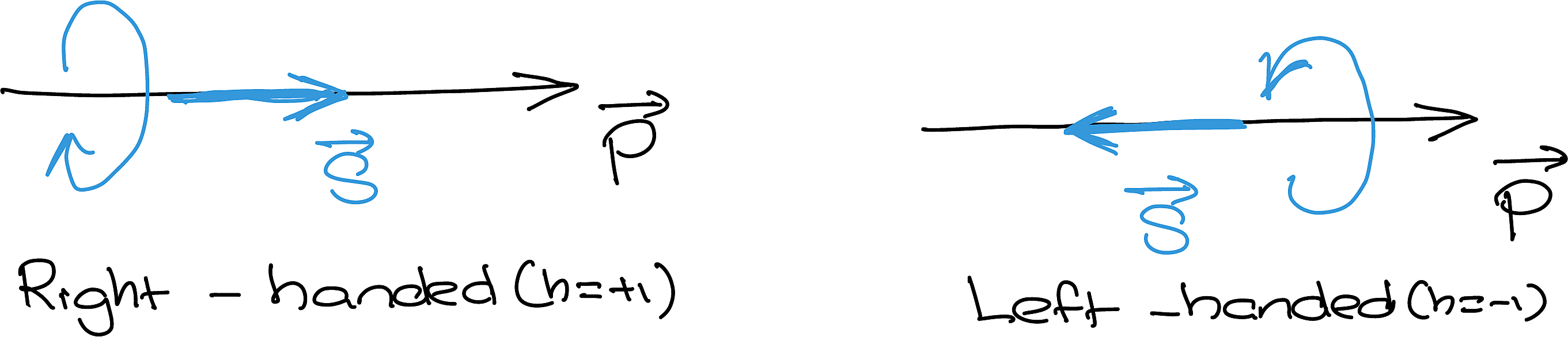
We can associate a property called helicity with a particle that carries spin \(\mathbf S\) and linear momentum \(\mathbf p\). For a spin-\(1/2\) particle, a convenient normalised definition is
\[ h = \dfrac{\v{p}\cdot \v{s}}{\left|\v{p}\cdot \v{s}\right|} \tag{7.12}\]
A helicity eigenstate has
\[ h=+1 \]
when its spin is aligned with its momentum, and
\[ h=-1 \]
when its spin is opposed to its momentum. These are called right-helicity and left-helicity states, respectively.
7.5.1 Helicity Depends on the Observer
For a massive particle, helicity is not Lorentz invariant. An observer moving faster than the particle can overtake it and then see its momentum pointing in the opposite direction. Its spin does not reverse, so the observer assigns the opposite helicity.
For a massless particle, no observer can overtake it. Its helicity is therefore Lorentz invariant. Neutrinos are not exactly massless, but in most experiments they are extremely relativistic. Helicity is consequently a very good practical description of their observed handedness.
The neutrinos we observe are typically travelling extremely close to the speed of light. For these highly relativistic particles:
7.5.2 A Brief Note About Chirality
The more fundamental form of handedness relevant to the weak interaction is chirality. Chirality is a quantum-field-theoretic property that describes how a fermion field transforms under Lorentz transformations. Unlike helicity, it is not defined by comparing the directions of a particle’s spin and momentum. However, for highly relativistic particles, chirality corresponds very closely to helicity.
The weak interaction distinguishes between the two chiralities. The charged weak interaction, mediated by \(W^\pm\), couples to left-chiral fermions and right-chiral antifermions. The neutral weak interaction, mediated by the \(Z^0\), couples to both left- and right-chiral charged fermion fields, but with different strengths. In the Standard Model, neutrinos participate in the weak interaction through their left-chiral components, while antineutrinos participate through their right-chiral components.
For a Dirac spinor, the chiral components are obtained using
\[ P_L=\frac{1-\gamma^5}{2}, \qquad P_R=\frac{1+\gamma^5}{2}, \]
so that
\[ \psi_L=P_L\psi, \qquad \psi_R=P_R\psi. \]
7.6 Parity Conservation and Parity Violation
7.6.1 Parity Is Mostly Conserved
The strong and electromagnetic interactions conserve parity. We can therefore use parity conservation to determine whether strong or electromagnetic processes are allowed and to deduce the parities of quantum states as we did in Example 7.1.
The weak interaction is different: it does not conserve parity. This means that a weak process and its parity-transformed counterpart need not occur with the same probability.
7.6.2 The Wu Experiment
In late 1956, Chien-Shiung Wu and her collaborators performed an experiment using the beta decay of polarised cobalt-60 nuclei. Their result, reported in 1957, provided the first direct experimental demonstration that parity is violated in the weak interaction.
The decay proceeds as
\[ \me{\ele{Co}{27}{60}{}} {\ele{Ni}{28}{60}{}^*+e^-+\bar\nu_e}, \tag{7.13}\]
followed by
\[ \me{\ele{Ni}{28}{60}{}^*} {\ele{Ni}{28}{60}{}+2\gamma}. \tag{7.14}\]
The beta decay leaves the nickel-60 nucleus in an excited state, indicated by the asterisk. The excited nucleus subsequently emits two gamma rays. These gamma rays were important experimentally because their angular distribution allowed the team to monitor how well the cobalt nuclei were aligned. However, they are not central to the parity argument itself.
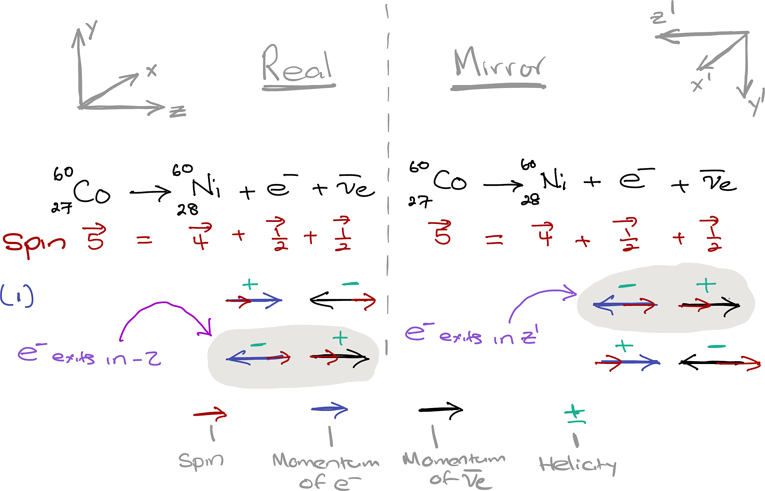
The cobalt-60 ground state has \(J^P=5^+\) and the relevant excited state of nickel-60 has \(J^P=4^+\).
Wu’s team cooled the sample to approximately \(0.01\,\mathrm{K}\) and placed it in a magnetic field. This caused a substantial fraction of the cobalt nuclear spins to align along a common axis. The essential parity argument can be expressed using two quantities:
- the nuclear spin, \(\mathbf J\), which is an axial vector and
- the electron momentum, \(\mathbf p_e\), which is a polar vector.
Under parity,
\[ \mathbf J\longrightarrow\mathbf J, \qquad \mathbf p_e\longrightarrow-\mathbf p_e. \]
Their scalar product therefore changes sign:
\[ \mathbf J\cdot\mathbf p_e \longrightarrow -\mathbf J\cdot\mathbf p_e. \tag{7.15}\]
If parity were conserved, the electron distribution would not favour one sign of \(\mathbf J\cdot\mathbf p_e\) over the other and electrons would have to be emitted parallel and antiparallel to the nuclear spin, about the same rate.
That is not what Wu and her collaborators observed. They found that electrons were emitted preferentially in the direction opposite to the cobalt nuclear spin. The original experiment and its parity-transformed counterpart therefore gave distinguishable predictions: nature was not indifferent to the transformation.
The nuclei could not be aligned perfectly, so the result was not that every electron emerged in one direction. Instead, the team measured a clear statistical asymmetry. The gamma-ray anisotropy provided an independent measure of the nuclear alignment, helping them distinguish the parity-violating signal from imperfect polarisation and other experimental effects.
We now understand this asymmetry as a consequence of the chiral structure of the charged weak interaction: it couples to left-chiral fermions and right-chiral antifermions.
For a historical account of the experiment, see NIST’s discussion of the reversal of the parity law.
For instance consider a superposition of an even parity and odd parity states.↩︎