11  Multipole Expansions*

\[ \newcommand\v[1]{\boldsymbol{#1}} \newcommand\vdot[2]{\v{#1}\cdot\v{#2}} \]

\[ \newcommand{\dd}[2][]{\mathrm{d}^{#1}#2} \]

\[ \newcommand\f[2]{\dfrac{#1}{#2}} \newcommand\da[2]{\dfrac{d #1}{d #2}} \newcommand\daa[2]{\dfrac{d^2 #1}{d #2^2}} \newcommand\pa[2]{\dfrac{\partial #1}{\partial #2}} \newcommand\pal[3]{\left.\dfrac{\partial #1}{\partial #2}\right|_{#3}} \newcommand\paa[2]{\dfrac{\partial^2 #1}{\partial #2^2}} \newcommand\pab[3]{\dfrac{\partial^2 #1}{\partial #2 \partial #3}} \def\half{\frac{1}{2}} \]

\[ \newcommand\ket[1]{\left|#1\right\rangle} % |x> \newcommand\exp[1]{\left\langle#1\right\rangle} % <x> \newcommand\lr[1]{\left(#1\right)} % (x) \newcommand\lrs[1]{\left[#1\right]} % [x] \newcommand\lra[1]{\left|#1\right|} % |x| \newcommand\lrc[1]{\left\{#1\right\}} % {x} \newcommand\lrl[3]{\left.#1\right|_{#2}^{#3}} % x_limits \]

\[ \def\ie{\text{i.e.}\quad} \]

\[ \newcommand{\me}[3][\rightarrow]{{#2}#1{#3}} % Typical reaction \newcommand{\nr}[3]{{#1}\,({#2})\,{#3}} % Nuclear reactions \newcommand{\ele}[4]{_{#2}^{#3}{\textbf{#1}}_{#4}} \newcommand{\el}[2]{^{#2}\text{#1}} \newcommand{\til}[2][\mathbf{\sim}]{\underset{#1}{{#2}}} \newcommand{\b}[1]{\overline{#1}} \]

\[ \newcommand{\coulomb}[1]{\dfrac{#1}{4\pi\epsilon_0}} \def\degree{^*} \]

\[ \def\amu{\text{ amu}} \def\J{\text{ J}} \def\K{\text{ K}} \def\s{\text{ s}} \def\second{\text{ s}} \def\Psecond{\text{ s}^{-1}} \def\m{\text{ m}} \def\mm{\text{ mm}} \def\km{\text{ km}} \def\fm{\text{ fm}} \def\mum{\text{ $\mu$m}} \def\mus{\text{ $\mu$s}} \def\mPERs{\text{ ms$^{-1}$}} \def\eV{\text{ eV}} \def\keV{\text{ keV}} \def\GeV{\text{ GeV}} \def\MeV{\text{ MeV}} \def\MeVc{\text{ MeV/c$^2$}} \def\KeVc{\text{ KeV/c$^2$}} \newcommand\ttp[1]{\times 10^{#1}} % To The Power \]

\[ \def\en{\nu_e} \def\Aen{\b{\nu_e}} \def\mun{\nu_\mu} \def\Amun{\b{\nu}_\mu} \]

\[ \def\uraniumA{\ele{U}{92}{233}{}} \def\uraniumB{\ele{U}{92}{235}{}} \def\uraniumC{\ele{U}{92}{238}{}} \def\carbonB{\ele{C}{6}{14}{}} \def\nitrogenB{\ele{N}{7}{14}{}} \def\oxygenA{\ele{O}{8}{14}{}} \def\oxygenB{\ele{O}{8}{16}{}} \]

\[ % \def\com{\text{\scriptsize CM}} \def\com{\mathrm{\scriptsize CM}} \]

\[ \def\l{l} \]

\[ \def\g{\gamma} \]

\[ \def\r{\v{r}} \def\rp{\v{r'}} \]

What to Expect in This Chapter

Unlike the strong and weak interactions, the electromagnetic interaction has an infinite range. Electromagnetic probes are especially valuable because their interactions with charge and current distributions are well understood and can be controlled experimentally. Consequently, much of what we know about nuclear structure comes from electromagnetic phenomena. In particular, electric and magnetic moments are among the quantities routinely measured and reported when describing a nucleus. These moments contain valuable information about the distributions of charge and current within it.

We will need these ideas later, particularly when we discuss \(\gamma\)-decay and how measurements of electromagnetic radiation reveal information about nuclei.

In this chapter, I will remind you of three important ideas that help us answer the following questions:

1. How can we understand the electric field produced by an arbitrary charge distribution?
2. How can we understand the magnetic field produced by an arbitrary current distribution?
3. How can we describe the radiation produced by time-dependent charge and current distributions?

The common thread connecting these questions is the multipole expansion.

11.1 Electric Moments

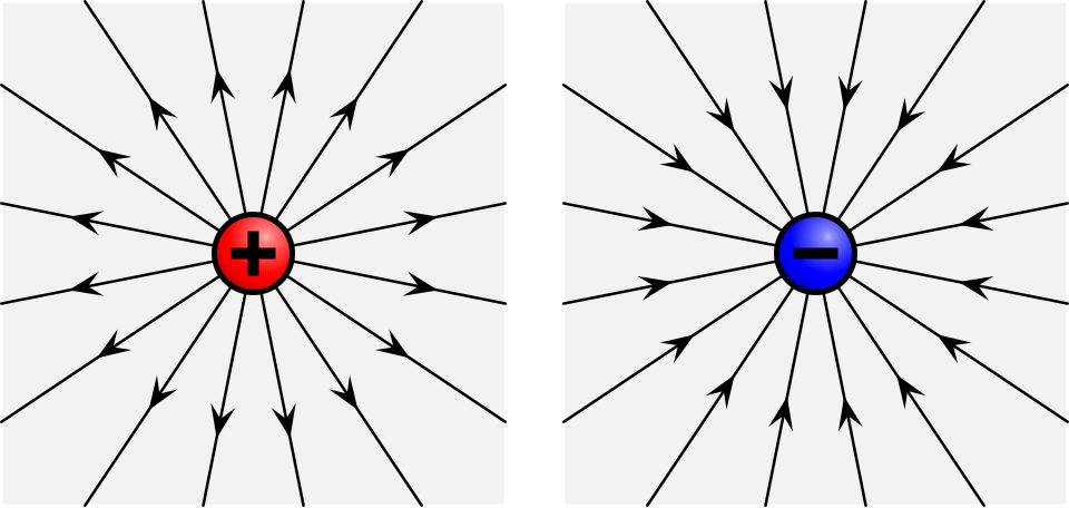
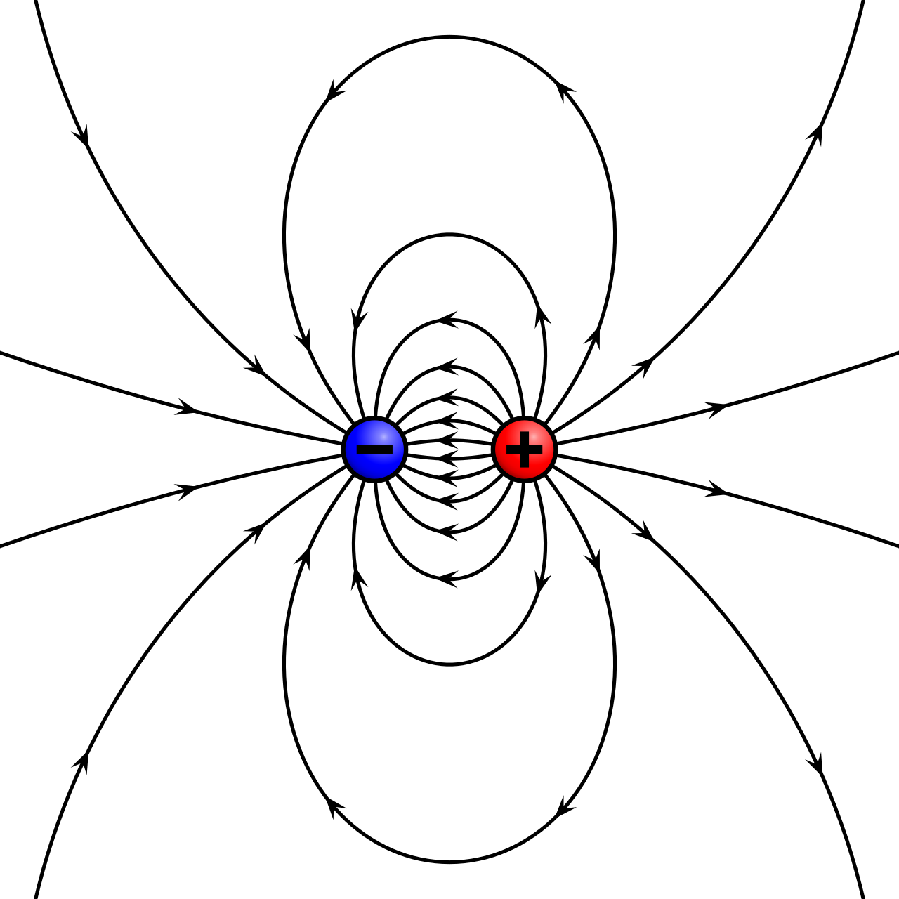
Recall that different charge distributions produce fields with characteristic spatial patterns. For example, the fields of a point charge and an electric dipole are shown alongside.

Even when we are far away and cannot directly ‘see’ the charge distribution, we can distinguish these two sources by examining their fields. The field of a point charge falls as \(1/r^2\) and is spherically symmetric, whereas the dipole field falls more rapidly, as \(1/r^3\), and has an angular dependence.

The general idea I am getting at is that we can learn about an unseen charge distribution by observing how its field varies far from the source.

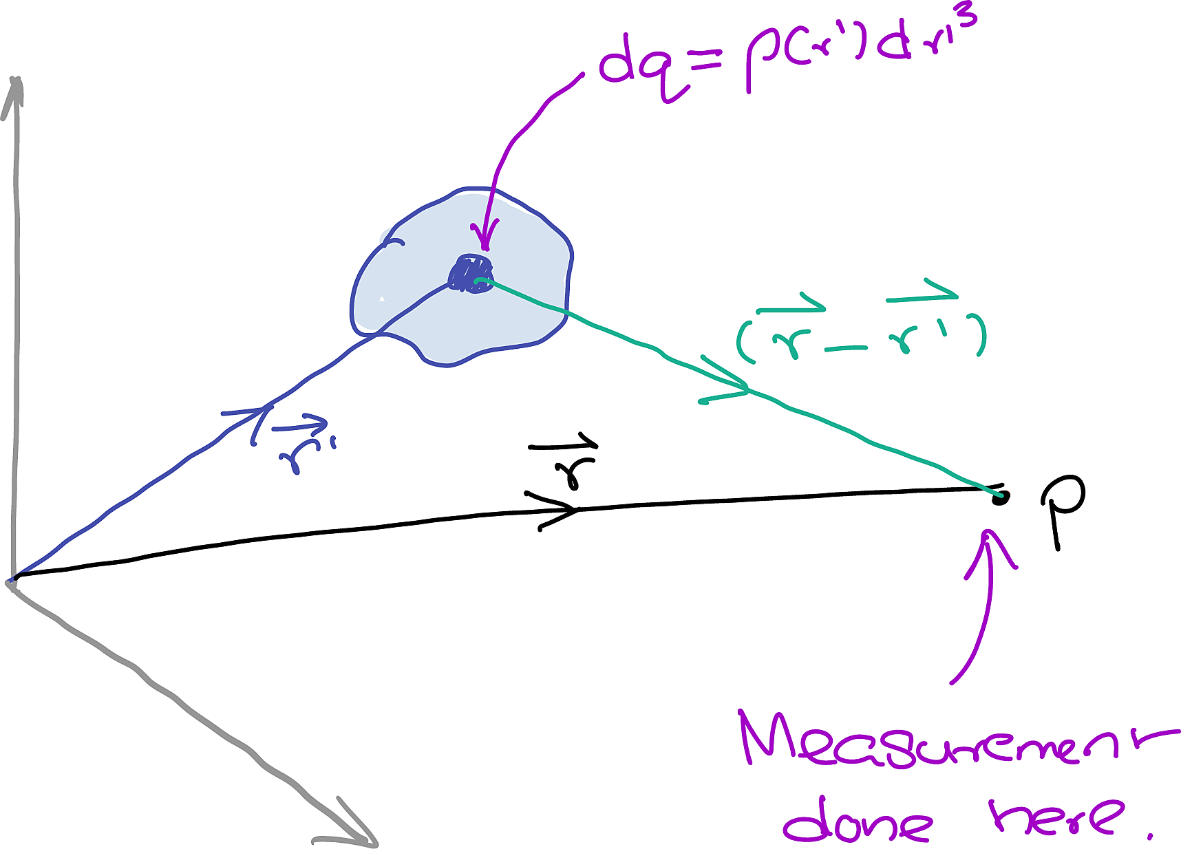
Let us make this argument more quantitative. Consider a charge distribution \(\rho(\v{r}')\). The electric potential at the observation point \(\v{r}\) is

\[ \Phi(\v{r}) = \frac{1}{4\pi\epsilon_0} \int \frac{\rho(\v{r}')}{|\v{r}-\v{r}'|} \,d^3r'. \tag{11.1}\]

The potential energy of a test charge \(q\) placed at \(\v{r}\) would be \(U=q\Phi\).

Let \(\gamma\) be the angle between \(\v{r}\) and \(\v{r}'\). Then, \[ \begin{align} |\r-\rp| &= \sqrt{r^2+r'^2 - 2\r\cdot\rp} \\ &= r\sqrt{1 + \underbrace{\lr{\f{r'}{r}}^2 - 2\lr{\f{r'}{r}}\cos\gamma }_{\Large\epsilon}}\\ &= r(1 + \epsilon)^{1/2} \end{align} \tag{11.2}\]

Far from the source, \(r\gg r',\) so \(r'/r\) is small and so if \(\epsilon\). We may therefore expand the denominator in powers of \(r'/r\) using the Binomial expansion:

\[ \begin{align} \f{1}{|\r-\rp|} &= \f{1}{r}\lr{1+\epsilon}^{-1/2} \\ &=\f{1}{r}\lr{1-\f{1}{2}\epsilon+\f{3}{8}\epsilon^2-\f{15}{16}\epsilon^3+\ldots} \end{align} \tag{11.3}\]

\[ \frac{1}{|\v{r}-\v{r}'|} = \frac{1}{r} \sum_{L=0}^{\infty} \left(\frac{r'}{r}\right)^L P_L(\cos\gamma), \tag{11.4}\]

where \(P_L\) is a Legendre polynomial. Keeping the first few terms gives

\[ \begin{aligned} \Phi(\v{r}) \approx \frac{1}{4\pi\epsilon_0} \Bigg[& \frac{1}{r}\int\rho(\v{r}')\,d^3r' \\ &+\frac{1}{r^2} \int\rho(\v{r}')r'\cos\gamma\,d^3r' \\ &+\frac{1}{2r^3} \int\rho(\v{r}')r'^2 \left(3\cos^2\gamma-1\right)d^3r' \\ &+\frac{1}{2r^4} \int\rho(\v{r}')r'^3 \left(5\cos^3\gamma-3\cos\gamma\right)d^3r' +\cdots\Bigg]. \end{aligned} \tag{11.5}\]

Simplifying and collecting like powers of \(\f{1}{r}\) yields:

\[ \begin{array}{llcc} U(\r) \approx &\displaystyle\f{k}{r}\int\rho(\rp)d^3r' & & \text{(Monopole)}\\ &+ \displaystyle\f{k}{r^2}\int\rho(\rp)\rp \, \lr{\cos\theta}\,d^3r' & & \text{(Dipole)}\\ &+ \displaystyle\f{k}{2r^3}\int\rho(\rp)\rp^2 \, \lr{{3}\cos^2\theta-{1}}\,d^3r' & & \text{(Quadrupole)}\\ &+ \displaystyle\f{k}{2r^4}\int\rho(\rp)\rp^3 \, \lr{{5}\cos^3\theta-{3}\cos\theta}\,d^3r' & & \text{(Octupole)}\\ &+ \cdots \end{array} \tag{11.6}\]

The successive terms are called the monopole, dipole, quadrupole and octupole terms.

The monopole term tells us the total charge. The dipole term describes the first departure from a point-like distribution, while the quadrupole and higher moments reveal progressively more detailed information about the shape of the charge distribution.

Higher-order terms fall more rapidly with distance. Therefore, far from the source, the first non-zero multipole usually dominates.

The multipole expansion does not replace the original charge distribution. It provides an increasingly accurate description of its field when the observation point is far from the source.

11.2 Magnetic Moments

\[ \def\mm{\v{\mu}} \]

Magnetic fields can be treated in a similar way by expanding the magnetic vector potential \(\v{A}\) produced by a current distribution.

\[ \begin{array}{llcc} \v{A} \approx &\f{\mu_0 I}{4\pi}\Bigr[\cancel{\displaystyle\f{1}{r}\oint d\v{l}} & & \text{(Monopole)}\\ &+ \displaystyle\f{1}{r^2}\oint\rp \, \cos\theta \,d\v{l} & & \text{(Dipole)}\\ &+ \displaystyle\f{1}{2r^3}\oint\rp^2 \, \lr{{3}\cos^2\theta-{1}}\,d\v{l} & & \text{(Quadrupole)}\\ &+ \cdots \Bigr] \end{array} \tag{11.7}\]

Notice an important difference. Electric charge can provide a monopole term, but isolated magnetic monopoles have not been observed. For a steady current, the current paths form closed loops, and the leading magnetic contribution is therefore the magnetic dipole.

11.2.1 \(\mu\) for a Circular Current

Classically

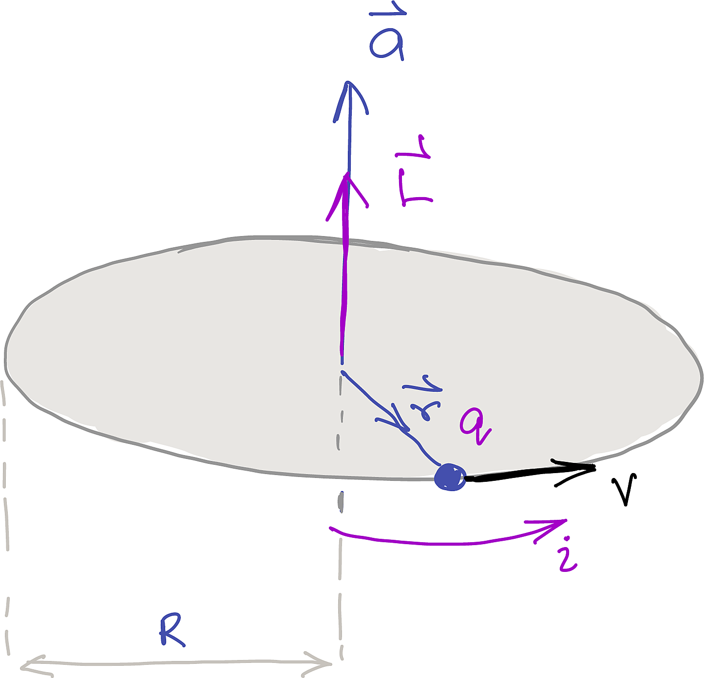
Let us consider a simple example to get a feel for \(\mm\). A circular loop carrying a current \(i\) and enclosing an area vector \(\v{a}\) has a magnetic dipole moment

\[ \mm=i\v{a}. \tag{11.8}\]

Suppose that the current is produced by a single charge \(q\) moving around a circular path of radius \(R\) with speed \(v\). Then,

\[ i = q\times\text{revolutions per second} = q\left(\frac{v}{2\pi R}\right). \tag{11.9}\]

The orbital angular momentum is

\[ \v{L} = mvR\,\hat{\v{a}}, \tag{11.10}\]

where \(\hat{\v{a}}\) points perpendicular to the plane of the orbit. Since \(\v{a}=\pi R^2\hat{\v{a}}\), it follows that

\[ { \mm=\frac{q}{2m}\v{L} }. \tag{11.11}\]

The quantity \(q/(2m)\) is the classical orbital gyromagnetic ratio. For an electron, \(q=-e\), so its magnetic moment points opposite to its orbital angular momentum. The magnitude of the corresponding ratio is \(e/(2m_e)\).

The main point I would like you to take away from this example is that the magnetic dipole moment is related to angular momentum. What we have discussed so far is only the contribution from orbital angular momentum. Intrinsic spin also contributes to the magnetic dipole moment.

11.3 From Multipole Moments to Multipole Radiation

So far, we have used multipole moments to describe static charge and current distributions. A monopole moment tells us the total charge, a dipole moment describes the first departure from a point-like source, and higher moments contain increasingly detailed information about the source.

The next step is to allow these moments to change with time.

A static electric dipole produces an electric field but does not radiate. An oscillating electric dipole, however, produces an electromagnetic radiation field. Similarly, an oscillating magnetic dipole produces magnetic-dipole radiation.

This gives us the connection we need:

• a time-dependent electric dipole produces \(E1\) radiation;
• a time-dependent magnetic dipole produces \(M1\) radiation;
• higher-order time-dependent moments produce \(E2\), \(M2\), \(E3\), \(M3\), and higher multipole radiation.

In nuclear physics, these labels describe the angular-momentum and parity properties of the photon emitted during a nuclear transition.

11.4 EM Radiation Due to a Pure Electric Dipole

Electromagnetic radiation is produced whenever a charge distribution changes in an appropriate way. The simplest place to start is with an oscillating electric dipole.

If you are wondering why we did not start with electric-monopole radiation, it is because a spherically symmetric oscillation of a fixed total charge does not produce a radiation field. The easiest way to see this is to draw a Gaussian surface around a charged sphere whose radius is oscillating. Even though the charge distribution oscillates, you will see no time variation in the field on the surface! Consequently, there is no photons associated with an \(E0\) transition.

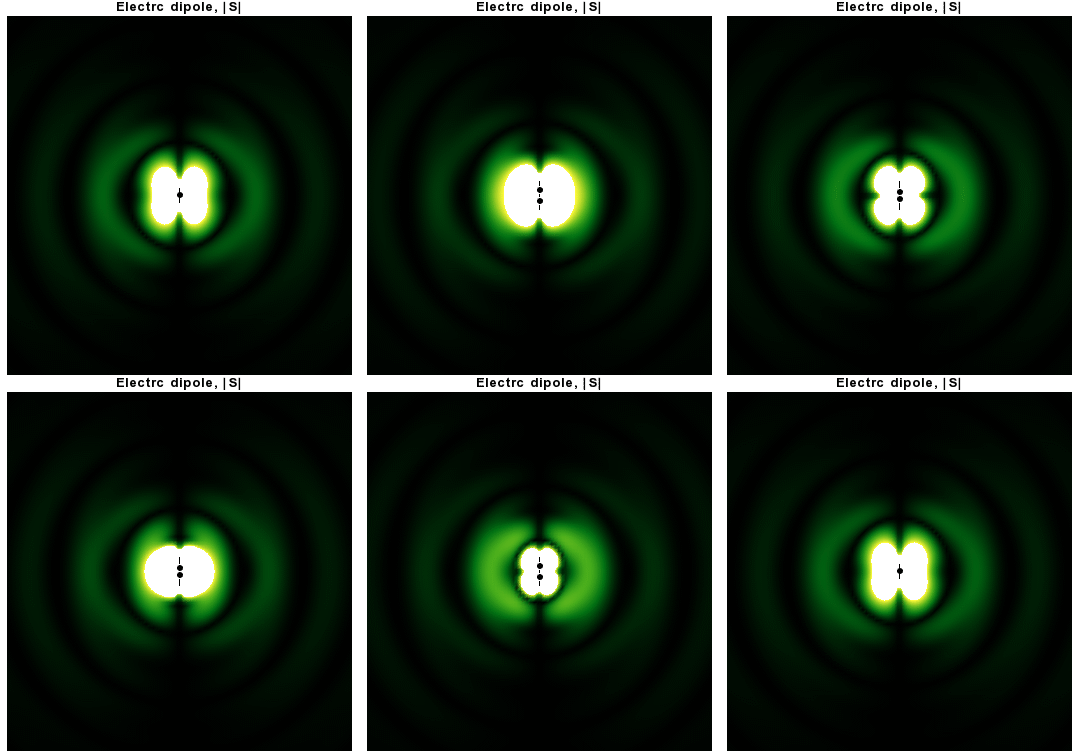
An electric dipole consists of charges \(-q_0\) and \(+q_0\) separated by a displacement \(\v{s}\). Its electric dipole moment is

\[ \v{p}_0=q_0\v{s}. \tag{11.12}\]

If the dipole oscillates with angular frequency \(\omega\), we may write

\[ \v{p}(t)=\v{p}_0\cos\omega t. \tag{11.13}\]

Starting from Maxwell’s equations, we can obtain the electric field, magnetic field and Poynting vector produced by the oscillating dipole. In the far-field region, the radiation fields are

\[ \begin{aligned} \v{E}(\v{r},t) &= -\frac{\mu_0p_0\omega^2}{4\pi} \frac{\sin\theta}{r} \cos\left[\omega\left(t-\frac{r}{c}\right)\right] \hat{\theta}, \\[3pt] \v{B}(\v{r},t) &= -\frac{1}{c} \frac{\mu_0p_0\omega^2}{4\pi} \frac{\sin\theta}{r} \cos\left[\omega\left(t-\frac{r}{c}\right)\right] \hat{\phi}. \end{aligned} \tag{11.14}\]

The time-averaged Poynting vector is

\[ \left\langle\v{S}\right\rangle = \frac{\mu_0p_0^2\omega^4}{32\pi^2c} \frac{\sin^2\theta}{r^2}\hat{r}. \tag{11.15}\]

There are several things to notice:

• These expressions describe the fields far from the dipole.
• Both fields fall as \(1/r\).
• The energy flux therefore falls as \(1/r^2\), as expected from the inverse-square law.
• The radiation has the characteristic angular distribution \(\sin^2\theta\).
• No energy is radiated along the dipole axis, while the intensity is greatest perpendicular to it.

Radiation produced by an electric dipole is called \(E1\) radiation. Here, \(E\) means electric and \(L=1\) identifies the dipole order.

11.5 Radiation Due to a Pure Magnetic Dipole

We can also produce radiation by allowing a current distribution to vary with time. The simplest magnetic source is an oscillating magnetic dipole, such as a small loop carrying an oscillating current.

If its magnetic dipole moment is

\[ \v{m}(t)=\v{m}_0\cos\omega t, \tag{11.16}\]

then the far-field radiation has the same characteristic \(\sin^2\theta\) angular distribution as electric-dipole radiation, but the orientations of the electric and magnetic fields are interchanged:

\[ \begin{aligned} \v{E}(\v{r},t) &= -\frac{\mu_0m_0\omega^2}{4\pi c} \frac{\sin\theta}{r} \cos\left[\omega\left(t-\frac{r}{c}\right)\right] \hat{\phi}, \\[3pt] \v{B}(\v{r},t) &= -\frac{\mu_0m_0\omega^2}{4\pi c^2} \frac{\sin\theta}{r} \cos\left[\omega\left(t-\frac{r}{c}\right)\right] \hat{\theta}. \end{aligned} \tag{11.17}\]

The corresponding time-averaged energy flux is

\[ \left\langle\v{S}\right\rangle = \frac{\mu_0m_0^2\omega^4}{32\pi^2c^3} \frac{\sin^2\theta}{r^2}\hat{r}. \tag{11.18}\]

Radiation produced by a magnetic dipole is called \(M1\) radiation. Here, \(M\) means magnetic and \(L=1\) again identifies the dipole order.

11.6 Generalisation to Higher Multipoles

The next electric multipole after the dipole is the quadrupole. An oscillating electric quadrupole produces \(E2\) radiation. We can similarly have \(E3\) octupole radiation, \(E4\) hexadecapole radiation and so on.

The magnetic sequence proceeds in the same way: \(M1\), \(M2\), \(M3\), and higher magnetic multipoles.

We can summarise the notation as follows:

• \(E\) or \(M\) identifies whether the radiation is electric or magnetic;
• \(L=1\) corresponds to dipole radiation;
• \(L=2\) corresponds to quadrupole radiation;
• \(L=3\) corresponds to octupole radiation;
• the photon carries total angular momentum with quantum number \(L\).

The label \(L\) specifies the total angular momentum of the multipole radiation about the source. It is not simply the spin of the photon.

Higher multipoles are usually less probable than lower multipoles.

Roughly speaking, each increase in multipole order introduces additional powers of the small quantity

\[ kR=\frac{E_\gamma R}{\hbar c}, \tag{11.19}\]

where \(R\) is the nuclear radius. Since nuclear dimensions are usually much smaller than the wavelength of the emitted \(\gamma\)-ray, \(kR\) is generally small. Therefore, the lowest-order multipole allowed by angular momentum and parity usually dominates.

More than one multipole may sometimes satisfy the selection rules. For example, a transition may contain a mixture of \(M1\) and \(E2\) radiation.

11.7 What Angular Momentum Does the Photon Carry?

At this point, you may be wondering how a spin-1 photon can carry the angular momentum associated with an \(E2\), \(M2\), \(E3\), or higher transition.

A real photon has only two physical polarisation states, corresponding to helicities \(+1\) and \(-1\). There is no physical longitudinal-polarisation state for a free photon.

However, radiation emitted by a localised source also has a spatial structure. The complete photon field can therefore carry total angular momentum with quantum number

\[ L=1,2,3,\ldots \]

about the source. The label \(L\) in \(EL\) or \(ML\) refers to this total angular momentum of the multipole radiation field. It should not be identified with the photon spin alone.

For example:

• \(E1\) and \(M1\) radiation have \(L=1\);
• \(E2\) and \(M2\) radiation have \(L=2\);
• \(E3\) and \(M3\) radiation have \(L=3\).

In this setting, separating the photon’s total angular momentum into independent spin and orbital parts is not always straightforward or unique.

11.8 Multipole Radiation, Quantum Mechanically

Consider a system with an initial nuclear state

\[ |i\rangle=|J_i,\eta_i\rangle \]

and a final nuclear state

\[ |f\rangle=|J_f,\eta_f\rangle, \]

where \(J\) and \(\eta\) represent the angular momentum and parity of each state, respectively.

Quantum mechanics allows an electromagnetic transition between these states through an appropriate multipole operator, such as \(E1\), \(M1\), \(E2\) or \(M2\).

11.8.1 Energy

In this process, a photon is emitted to conserve energy:

\[ E_\gamma=\hbar\omega=E_i-E_f. \tag{11.20}\]

11.8.2 Angular Momentum

The multipole order \(L\) specifies the total angular momentum carried by the photon. Angular-momentum conservation requires

\[ { |J_i-J_f| \leq L \leq J_i+J_f }. \tag{11.21}\]

A single photon cannot connect two states that both have zero angular momentum:

\[ J_i=0\rightarrow J_f=0 \qquad \text{is forbidden for one-photon emission.} \tag{11.22}\]

11.8.3 Parity

Electromagnetic interactions also conserve parity. However, electric and magnetic multipole operators transform differently under spatial inversion.

To understand how this works, recall that the \(E1\) transition amplitude depends on the matrix element

\[ \langle f|\hat{p}_e| i\rangle = q_0\langle f|\hat{r}| i\rangle. \]

From the point of view of the spatially inverted system, this matrix element becomes

\[ q_0\langle f'|-\hat{r}| i'\rangle, \]

where I have used the prime (\('\)) to indicate the spatially inverted wavefunctions.

Since the states have definite parity,

\[ \ket{i'}=\eta_i \ket{i} \qquad\text{and}\qquad \ket{f'}=\eta_f \ket{f}. \]

The matrix element can therefore be non-zero only if

\[ \eta_f\eta_i=-1. \]

In other words, an \(E1\) transition can occur only between states of opposite parity.

More generally, for an electric multipole transition \(EL\),

\[ { \eta_f=\eta_i(-1)^L }. \tag{11.23}\]

For a magnetic multipole transition \(ML\),

\[ { \eta_f=\eta_i(-1)^{L+1} }. \tag{11.24}\]

The most common cases are summarised below:

Transition	Multipole order	Parity relation
\(E1\)	\(L=1\)	Parity changes
\(M1\)	\(L=1\)	Parity does not change
\(E2\)	\(L=2\)	Parity does not change
\(M2\)	\(L=2\)	Parity changes

11.9 Bringing the Ideas Together

The multipole expansion gives us a common language for describing both nuclear structure and electromagnetic transitions:

• Static electric and magnetic moments tell us about nuclear charge and current distributions.
• Time-dependent moments produce electromagnetic radiation.
• The multipole label \(EL\) or \(ML\) tells us the type and angular momentum of the emitted radiation.
• Angular-momentum and parity conservation determine which transitions are allowed.
• When several transitions are allowed, the lowest multipole order usually dominates.

These ideas will allow us to interpret nuclear \(\gamma\)-decay schemes and use electromagnetic radiation to learn about the spin, parity and structure of nuclear states.