2 A Whirlwind Tour of Special Relativity*
\[ \newcommand\v[1]{\boldsymbol{#1}} \newcommand\vdot[2]{\v{#1}\cdot\v{#2}} \]
\[ \newcommand{\dd}[2][]{\mathrm{d}^{#1}#2} \]
\[ \newcommand\f[2]{\dfrac{#1}{#2}} \newcommand\da[2]{\dfrac{d #1}{d #2}} \newcommand\daa[2]{\dfrac{d^2 #1}{d #2^2}} \newcommand\pa[2]{\dfrac{\partial #1}{\partial #2}} \newcommand\pal[3]{\left.\dfrac{\partial #1}{\partial #2}\right|_{#3}} \newcommand\paa[2]{\dfrac{\partial^2 #1}{\partial #2^2}} \newcommand\pab[3]{\dfrac{\partial^2 #1}{\partial #2 \partial #3}} \def\half{\frac{1}{2}} \]
\[ \newcommand\ket[1]{\left|#1\right\rangle} % |x> \newcommand\exp[1]{\left\langle#1\right\rangle} % <x> \newcommand\lr[1]{\left(#1\right)} % (x) \newcommand\lrs[1]{\left[#1\right]} % [x] \newcommand\lra[1]{\left|#1\right|} % |x| \newcommand\lrc[1]{\left\{#1\right\}} % {x} \newcommand\lrl[3]{\left.#1\right|_{#2}^{#3}} % x_limits \]
\[ \def\ie{\text{i.e.}\quad} \]
\[ \newcommand{\me}[3][\rightarrow]{{#2}#1{#3}} % Typical reaction \newcommand{\nr}[3]{{#1}\,({#2})\,{#3}} % Nuclear reactions \newcommand{\ele}[4]{_{#2}^{#3}{\textbf{#1}}_{#4}} \newcommand{\el}[2]{^{#2}\text{#1}} \newcommand{\til}[2][\mathbf{\sim}]{\underset{#1}{{#2}}} \newcommand{\b}[1]{\overline{#1}} \]
\[ \newcommand{\coulomb}[1]{\dfrac{#1}{4\pi\epsilon_0}} \def\degree{^*} \]
\[ \def\amu{\text{ amu}} \def\J{\text{ J}} \def\K{\text{ K}} \def\s{\text{ s}} \def\second{\text{ s}} \def\Psecond{\text{ s}^{-1}} \def\m{\text{ m}} \def\mm{\text{ mm}} \def\km{\text{ km}} \def\fm{\text{ fm}} \def\mum{\text{ $\mu$m}} \def\mus{\text{ $\mu$s}} \def\mPERs{\text{ ms$^{-1}$}} \def\eV{\text{ eV}} \def\keV{\text{ keV}} \def\GeV{\text{ GeV}} \def\MeV{\text{ MeV}} \def\MeVc{\text{ MeV/c$^2$}} \def\KeVc{\text{ KeV/c$^2$}} \newcommand\ttp[1]{\times 10^{#1}} % To The Power \]
\[ \def\en{\nu_e} \def\Aen{\b{\nu_e}} \def\mun{\nu_\mu} \def\Amun{\b{\nu}_\mu} \]
\[ \def\uraniumA{\ele{U}{92}{233}{}} \def\uraniumB{\ele{U}{92}{235}{}} \def\uraniumC{\ele{U}{92}{238}{}} \def\carbonB{\ele{C}{6}{14}{}} \def\nitrogenB{\ele{N}{7}{14}{}} \def\oxygenA{\ele{O}{8}{14}{}} \def\oxygenB{\ele{O}{8}{16}{}} \]
\[ % \def\com{\text{\scriptsize CM}} \def\com{\mathrm{\scriptsize CM}} \]
\[ \def\l{l} \]
\[ \def\g{\gamma} \]
\[ \def\p{p^\mu} \]
What To Expect In This Chapter
Many of the ideas in this course rest on concepts from relativity and quantum mechanics. In particular, several important features of particle reactions can be described and understood only through the lens of relativity. In this chapter, I will take you through a whirlwind tour of the essential ideas and tools from special relativity that we will use throughout the course.
2.1 Spacetime four-vectors
Special relativity is based on two postulates:
- The laws of physics have the same form in all inertial reference frames.
- The speed of light has the same value, \(c\), in all inertial reference frames.
Together, these postulates require space and time to be treated as parts of a single structure: spacetime. An event is represented by the spacetime four-vector
\[ a\equiv\left(a^{0},a^{1},a^{2},a^{3}\right) \equiv\left(ct,x,y,z\right) \tag{2.1}\]
Note following:
- \(c\) is the speed of light.
- The exponents (e.g. \(0\) in \(a^0\)) is an index/label, not a power.
- The first component is related to time (\(a^0 = ct\)), and the rest (\(a^{1}=x\), \(a^{2}=y\), \(a^{3}=z\)) are the spatial coordinates.
Because it contains both spatial and temporal information, this is called the spacetime four-vector.
2.2 Scaler product of four vectors
The scalar product1 of two four-vectors is defined as:
\[ a \cdot b=a^{0}b^{0}-a^{1}b^{1}-a^{2}b^{2}-a^{3}b^{3} \tag{2.2}\]
Notice that we can also rewrite Equation 2.2 so that the spatial portion is given by the familiar vector scalar product \(\vdot{a}{b}\):
\[ a\cdot b=a^{0}b^{0}-\v{a}\cdot \v{b} \tag{2.3}\]
This scalar product is Lorentz invariant. In other words, all inertial observers obtain the same value for \(a\cdot b\), even though might disagree about the individual components of \(a\) and \(b\).
2.3 Energy-momentum four-vector
The four-vector most relevant to particle physics is the energy–momentum four-vector, which we denote by \(\p\):
\[ \p\equiv\left(\dfrac{E}{c},p_{x},p_{y},p_{z}\right) \tag{2.4}\]
Here, \(E\) is the particle’s total relativistic energy and \(\v{p}\) is its three-momentum. For a particle of rest mass \(m\) moving with velocity \(\v{v}\),
\[ E=\gamma mc^{2} \tag{2.5}\]
and
\[ \v{p}=\gamma m\v{v} \tag{2.6}\]
Where \(m\) is the rest-mass and
\[ \gamma =\frac{1}{\sqrt{1-\dfrac{v^{2}}{c^{2}}}}. \tag{2.7}\]
We don’t need to know how to derive the above for our present work. We just need to understand what they mean and how to use them. However, if you like, please refer to1 for a quick introduction.
2.4 Invariance
One of the most useful properties of four-vectors is that their scalar product is Lorentz invariant. Consequently, the squared norm (\(a^2\)) of any four-vector (including a sum or difference of four-vectors) has the same value in every inertial reference frame. A particularly useful example is the squared norm of the energy–momentum four-vector:
\[ (\p)^{2}=\p.\p=\left( \frac{E}{c}\right) ^{2}-p_{x}^{2}-p_{y}^{2}-p_{z}^{2}=\left( \frac{E}{c}\right) ^{2}-\v{p}^{2} \]
If we now substitute the expressions for \(E\) and \(p\) from equations Equation 2.5 and Equation 2.6, we get
\[ p^{2}=\left( \frac{E}{c}\right) ^{2}-\v{p}^{2}=m^{2}c^{2} \tag{2.8}\]
There are three important things I would like to highlight and re-iterate.
- Reorganising the right portion of Equation 2.8 yields the familiar:
\[ E^2 = \lra{\v{p}}^2c^2 + m^2c^4 \tag{2.9}\]
A particle at rest (\(\v{p} = \v{0}\)) will have an energy given by: \[ E=mc^2 \tag{2.10}\] This energy is called rest energy of the particle and is associated with its rest mass.
The third (and more cool feature) is that \(p^2\) is invariant! So, if two observers in two different (inertial) frames of reference look at the particle and calculate \(p^2\), they will get the same number!
So, I can write
\[ \underbrace{\left(\frac{E_{1}}{c}\right) ^{2}-\v{p_{1}}^{2}=p_{1}^{2}}_{\text{Frame 1}}=m^{2}c^{2}=\underbrace{p_{2}^{2}=\left(\frac{E_{2}}{c}\right) ^{2}-\v{p_{2}}^{2}}_{\text{Frame 2}} \tag{2.11}\]
You will see that this is an invaluable tool for understanding many, many things in nuclear and particle physics. This is a good place to remind ourselves that:
Now let me show you how to use these ideas in some situations related to particle physics.
2.5 Worked Examples I
Example 2.1 It is known that the following reaction can occur:
\[ \me{p+p}{p+p+p+\b{p}} \tag{2.12}\]
We’d like to know the minimum energy for this reaction to occur. i.e. we’d like to know how much energy we must impart on one proton so that the reaction will proceed. We note that at the minimum threshold energy (\(E_\text{th}\)), the four products will just be created with no additional energy left for motion when viewed in the CM frame. The situation is shown in the figure below.
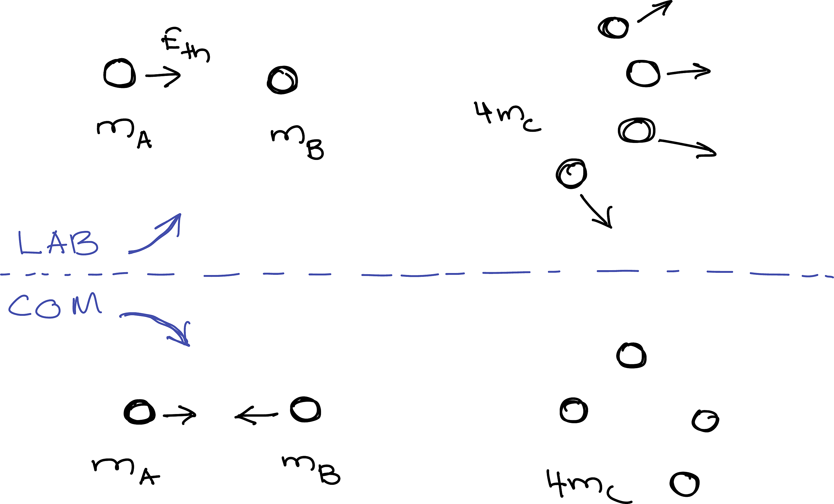
I have shown both the LAB frame and the CM frame. In the CM frame, at the threshold energy, the products are stationary immediately after the reaction.
To analyse this reaction, I will exploit the invariance of \(p^2\) for the total energy-momentum four-vector.
Since energy and momentum are conserved, we can write the following for the total energy-momentum four-vector \(p\) for the system
\[ \begin{align} \p_\text{\scriptsize AFTER(LAB)} &= \p_\text{\scriptsize BEFORE(LAB)}\\ \p_\text{\scriptsize AFTER(CM)} &= \p_\text{\scriptsize BEFORE(CM)}\\ \end{align} \tag{2.13}\]
Additionally, since \(p^2\) is invariant,
\[ (\p_\text{\scriptsize LAB})^2 = (\p_\text{\scriptsize CM})^2 \tag{2.14}\]
Leading to:
\[ (\p_\text{\scriptsize BEFORE(LAB)})^2= (\p_\text{\scriptsize AFTER(CM)})^2 \tag{2.15}\]
But,
\[ \begin{align*} \p_\text{\scriptsize BEFORE(LAB)}&=\left(\dfrac{E_{th}+m_{B}c^{2}}{c},\v{p}_{A} ,0,0\right) \\ \p_\text{\scriptsize AFTER(CM)}&=\left( \dfrac{4m_{C}c^{2}}{c},0,0,0\right) \end{align*} \tag{2.16}\]
I have retained the labelling of the protons \(A\), \(B\) and \(C\). This will help you keep track of where each appears in the equations.
Substituting Equation 2.16 in Equation 2.15 gives:
\[ \lr{\f{E_{th}+m_{B}c^{2}}{c}}^{2}- \v{p}_{A}^2=16m_{C}^{2}c^{2} - 0 \]
Note that \(E_{th}\) also includes the rest-energy \(m_Ac^2\) of proton \(A\).
Applying Equation 2.8 only to proton \(A\) yields:
\[ -\v{p}_{A}^2 = m_A^2c^2 - \lr{\f{E_{th}}{c}}^2 \]
Whence,
\[ \left(\dfrac{E_{th}+m_{B}c^{2}}{c}\right)^{2}+\left[m_{A}^{2}c^{2}-\left(\dfrac{E_{th}}{c}\right)^{2}\right]=16m_{C}^{2}c^{2} \]
We no longer need to distinguish between the protons. So, I will drop the labels \(A,B,C\) and simplify.
\[\begin{align} \lr{E_{th} + mc^2}^2 + m^2c^4 - E_{th}^2 &= 16m^2c^4 \\ 2E_{th}\,mc^2 + 2m^2c^4&= 16m^2c^4 \\ \Rightarrow E_{th} &= 7 mc^2 \end{align}\]
So, we must shoot the proton with a kinetic energy of at least \(6\,m_p\)! This is despite creating only two additional \(m_p\) masses at the end. Why is there such a waste of energy?
Example 2.2 Consider particle \(A\) that decays into two products \(B\) and \(C\) as indicated below.
\[A\rightarrow B+C\]
We want to know the kinetic energy \(E_C\) of the decay product \(C\).
We immediately see from the law of conservation of momentum that \[ \v{p}_{B} =-\v{p}_{C} \]
Further, since the energy-momentum four-vector is conserved:
\[ \begin{align} \p_{A}&=\p_{B}+\p_{C}\\ \p_{B}&=\p_{A}-\p_{C}\\ \Rightarrow p_{B}^{2}&=p_A^{2}+ p_{C}^{2} -2p_{A}\cdot p_{C}\\ \end{align} \tag{2.17}\]
But, using Equation 2.8 separately for each particle,
\[\begin{align} \p_{A}&=\lr{\f{m_Ac^2}{c}, \v{0}} \Rightarrow (\p_{A})^2 =m_{A}^2c^2\\ \p_{B}&=\lr{\f{E_B}{c}, \v{p}_{B}} \Rightarrow (\p_{B})^2 = \lr{\f{E_{B}}{c}}^2 - \v{p}_{B}^2 =m^2_Bc^2\\ \p_{C}&=\lr{\f{E_C}{c}, \v{p}_{C}} \Rightarrow (\p_{C})^2 = \lr{\f{E_{C}}{c}}^2 - \v{p}_{C}^2 =m^2_Cc^2 \end{align}\]
We can also use Equation 2.2 with \(\p_A\) and \(\p_C\):
\[ \p_{A}\cdot \p_{C}=\left(\dfrac{E_A}{c}\right)\left(\dfrac{E_C}{c}\right) - \v{0}\cdot\v{p}_{C} = \left(\dfrac{m_{A}c^{2}}{c}\right) \left(\dfrac{E_C}{c}\right) =m_A E_C \]
Substituting all these in Equation 2.17, gives:
\[ m^2_{B}c^2 = m^2_{A}c^2+ m^2_{C}c^2 - 2m_A E_C \]
Which leads to: \[ E_C = \left(\dfrac{m^2_{A} - m^2_{B} + m^2_{C}}{2m_A}\right)c^2 \tag{2.18}\]
Looking ahead: A striking feature of this result is that for a reaction with only two products, the kinematics leads to a single, unique energy for the outgoing particle \(C\). This energy is only determined by the masses of the various actors \(A\), \(B\) and \(C\). This observation was critical to the discovery of the neutrino.
2.6 Time Dilation
Another insight of special relativity that proves invaluable for particle physics is the phenomenon of time dilation. If a process requires a time interval \(\Delta t_\text{rest}\) in the rest frame, then the time elapsed for the same process in a different frame that is moving at speed \(v\) is lengthened or dilated, yielding:
\[ \Delta t_\text{other}=\gamma\Delta t_\text{rest} \tag{2.19}\]
2.7 Worked Examples II
Example 2.3 Before the advent of fancy particle accelerators, cosmic-rays were an invaluable source of high-energy particles. A significant constituent of the particle showers produced in the collision of cosmic-rays (mostly high-energy protons) with the upper atmosphere are muons that travel at almost the speed of light. The mass of these muons is about \(m_\mu=105.658\MeVc\) and the lifetime about \(\tau_\text{rest}=2.197\mus\).
This should mean these muons can only penetrate about: \[ 2.197\mus\times 2.9979\times10^8\mPERs = 658.4\m \]
down into the atmosphere. However, we find lots of muons at sea level!
This is possible because the muon lifetime is dilated in our frame-of-reference! Let’s make this a bit quantitative by looking at a \(2\GeV\) muon.
Using Equation 2.5 gives us:
\[ \gamma = \f{2\GeV}{105.658\MeVc \times c^2} = \f{2000}{105.658} \]
Hence, the life-time in our eyes is:
\[ \tau_\text{Earth} = \gamma \tau_\text{rest} = \f{2000}{105.658} \times 2.197\mus = 41.59\mus \]
So, the muons can actually travel:
\[ 41.59\mus\times 2.9979\times10^8\mPERs = 12.47\km \]
Example 2.4 Particles with lifetimes greater than \(10^{-13}\s\) are usually considered long-lived when compared with those that decay in time-scales of \(10^{-23}\s\)!
These long-life particles can be detected by observing their tracks because of time-dilation! Consider a long-lived particle with energy about 100 times that of its rest mass so that \(\gamma = 100\). Taking that these travel at almost the speed of light, the length of the track they leave in a detector will be:
\[ c\times(\gamma\times10^{-13}\s) \approx 3\mm \]
This length can easily be detected.
Unfortunately, even with time dilation helping, this method cannot detect the other short-lived particles because the tracks are far too small. Actually, ‘small’ is an understatement, as the tracks will be smaller than an atom!.
Chapter References
More precisely: the Minkowski scalar product↩︎