.just-for-now{
    background-color: rgba(255, 165, 0, 0.075);
}Worked Examples 1
\[ \newcommand\v[1]{\boldsymbol{#1}} \newcommand\vdot[2]{\v{#1}\cdot\v{#2}} \]
\[ \newcommand{\dd}[2][]{\mathrm{d}^{#1}#2} \]
\[ \newcommand\f[2]{\dfrac{#1}{#2}} \newcommand\da[2]{\dfrac{d #1}{d #2}} \newcommand\daa[2]{\dfrac{d^2 #1}{d #2^2}} \newcommand\pa[2]{\dfrac{\partial #1}{\partial #2}} \newcommand\pal[3]{\left.\dfrac{\partial #1}{\partial #2}\right|_{#3}} \newcommand\paa[2]{\dfrac{\partial^2 #1}{\partial #2^2}} \newcommand\pab[3]{\dfrac{\partial^2 #1}{\partial #2 \partial #3}} \def\half{\frac{1}{2}} \]
\[ \newcommand\ket[1]{\left|#1\right\rangle} % |x> \newcommand\exp[1]{\left\langle#1\right\rangle} % <x> \newcommand\lr[1]{\left(#1\right)} % (x) \newcommand\lrs[1]{\left[#1\right]} % [x] \newcommand\lra[1]{\left|#1\right|} % |x| \newcommand\lrc[1]{\left\{#1\right\}} % {x} \newcommand\lrl[3]{\left.#1\right|_{#2}^{#3}} % x_limits \]
\[ \def\ie{\text{i.e.}\quad} \]
\[ \newcommand{\me}[3][\rightarrow]{{#2}#1{#3}} % Typical reaction \newcommand{\nr}[3]{{#1}\,({#2})\,{#3}} % Nuclear reactions \newcommand{\ele}[4]{_{#2}^{#3}{\textbf{#1}}_{#4}} \newcommand{\el}[2]{^{#2}\text{#1}} \newcommand{\til}[2][\mathbf{\sim}]{\underset{#1}{{#2}}} \newcommand{\b}[1]{\overline{#1}} \]
\[ \newcommand{\coulomb}[1]{\dfrac{#1}{4\pi\epsilon_0}} \def\degree{^*} \]
\[ \def\amu{\text{ amu}} \def\J{\text{ J}} \def\K{\text{ K}} \def\s{\text{ s}} \def\second{\text{ s}} \def\Psecond{\text{ s}^{-1}} \def\m{\text{ m}} \def\mm{\text{ mm}} \def\km{\text{ km}} \def\fm{\text{ fm}} \def\mum{\text{ $\mu$m}} \def\mus{\text{ $\mu$s}} \def\mPERs{\text{ ms$^{-1}$}} \def\eV{\text{ eV}} \def\keV{\text{ keV}} \def\GeV{\text{ GeV}} \def\MeV{\text{ MeV}} \def\MeVc{\text{ MeV/c$^2$}} \def\KeVc{\text{ KeV/c$^2$}} \newcommand\ttp[1]{\times 10^{#1}} % To The Power \]
\[ \def\en{\nu_e} \def\Aen{\b{\nu_e}} \def\mun{\nu_\mu} \def\Amun{\b{\nu}_\mu} \]
\[ \def\uraniumA{\ele{U}{92}{233}{}} \def\uraniumB{\ele{U}{92}{235}{}} \def\uraniumC{\ele{U}{92}{238}{}} \def\carbonB{\ele{C}{6}{14}{}} \def\nitrogenB{\ele{N}{7}{14}{}} \def\oxygenA{\ele{O}{8}{14}{}} \def\oxygenB{\ele{O}{8}{16}{}} \]
\[ % \def\com{\text{\scriptsize CM}} \def\com{\mathrm{\scriptsize CM}} \]
\[ \def\l{l} \]
\[ \def\g{\gamma} \]
\[ \def\p{p^\mu} \newcommand{\cm}[2][\mathbf{\sim}]{\underset{#1}{{#2}}} \]
Q1 to Q3 (Geometric Preliminaries)
Solution 1.
A momentum vector in three dimensions can be written as: \(\v{p} = p_x \v{\hat{a}_x} + p_y \v{\hat{a}_y} + p_z\v{\hat{a}_z}.\)
If the magnitude is fixed, \(p = |\v{p}|\) then all allowed vectors satisfy \(p_x^2 + p_y^2 + p_z^2 = p^2.\)
This is the equation of a sphere of radius \(p\) in momentum space.
Alternatively:
If you move a vector of fixed size around its tip will trace out a sphere of radius \(|\v{p}|\). So, all stated descrivesd by \(\v p\) lies on this sphere.
Solution 2.
If \(p\) increases by a small amount \(\dd p\), the set of allowed momentum vectors expands from a sphere of radius \(p\) to one of radius \(p + \dd p\) in momentum space.
The additional states introduced by this increase lie in a thin spherical shell between \(p\) and \(p + \dd p\), with volume \(4\pi p^2\, \dd p\).
Hence, the number of states (or directions) available between \(p\) and \(p+\dd p\) is proportional to \(p^2\). \[ N(p) \propto p^2. \]
Solution 3.
If \(p_1\) and \(p_2\) are fixed in size such that \(p_2 = 2p_1\), then \[ \frac{N_2}{N_1} = \frac{p_2^2}{p_1^2} = 4. \]
So there are four times as many states.
Q4 & Q5 (Solid Angle)
Solution 4.
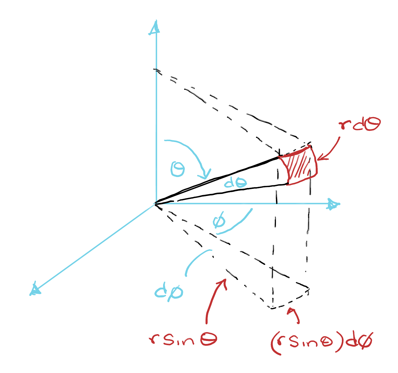
Lets start with \(\dd A\); from geometry of a sphere:
- arc length in \(\theta\) : \(r\,\dd\theta\)
- arc length in \(\phi\) : \(r\sin\theta\,\dd\phi\)
So the area element is \[ \dd A = r^2 \sin\theta\,\dd\theta\,\dd\phi. \]
Hence, \[ \dd\Omega = \frac{\dd A}{r^2} = \sin\theta\,\dd\theta\,\dd\phi. \]
Solution 5.
The total solid angle is obtained by integrating over all directions:
\[\begin{align} \Omega_{\max} &= \int_{\theta=0}^{\theta=\pi} \int_{\phi=0}^{2\pi} \sin\theta\,\dd\theta\,\dd\phi =\lr{\int_{\theta=0}^{\theta=\pi} \sin\theta\,\dd\theta} \lr{\int_{\phi=0}^{2\pi} \dd\phi} \\ &=\lrs{-\cos\theta}_0^\pi \;(2\pi)\;\\ &= 4\pi. \end{align}\]
Q6 & Q7 (Lorentz Invariants)
Solution 6. \[ s = (\p_1 + \p_2)^2={\p_1}^2 + {\p_2}^2 + 2 \p_1 \cdot \p_2 \]
Since, \[ \p = \left(\frac{E}{c}, \v{p}\right),\qquad\text{and}\qquad\p_a\cdot\p_b = \f{E_aE_b}{c^2} - \v{p_a}\cdot\v{p_b}, \]
we get, \[\begin{align} {\p_1}^2 &= \lr{\f{E_1}{c}}^2 - {p_1}^2\\ {\p_2}^2 &= \lr{\f{E_2}{c}}^2 - {p_2}^2\\ \p_1\cdot\p_2 &=\f{E_1E_2}{c^2} - \v{p_1}\cdot\v{p_2} \end{align}\]
Additionally,
\[ (\v{p}_1 + \v{p}_2)^2 = {p_1}^2 + 2\v{p_1}\cdot\v{p_2} + {p_2}^2 \]
Whence, \[ s c^2 = (E_1 + E_2)^2 - c^2 |\v{p}_1 + \v{p}_2|^2. \]
In the centre-of-mass frame, \[ \v{p}_1 + \v{p}_2 = \v{0}. \]
So \[ \sqrt{s}\,c = \cm{E_1} + \cm{E_2} = \cm{{E_\text{total}}}. \]
Alternatively:
In the centre of mass frame:
\[\begin{align} s = (\cm{\p_1} + \cm{\p_2})^2 &= \lr{\f{\cm{E_1} + \cm{E_2}}{c}, \underbrace{{\v{p}_1+\v{p}_2}}_{=\v{0}}}^2 \\ &= \lr{\f{\cm{E_1} + \cm{E_2}}{c}}^2 - 0\\ \Rightarrow \sqrt{s}\,c &= \cm{E_1} + \cm{E_2} . \end{align}\]
Solution 7.
At threshold the final particles have no kinetic energy in the COM frame and the total energy is purely rest mass \(mc^2\). So, \[ {{\cm{E}}_\text{total\,@\,threshold}}=\sqrt{s_{\text{th}}}\,c = (m_3 + m_4)c^2. \]
Q8 (Near-Threshold Behaviour)
Solution 8.
At threshold, the excess energy \(Q\) becomes kinetic energy.
Using non-relativistic approximation: \[ \cm{Q} = \frac{\cm{p}^2}{2m_3} + \frac{\cm{p}^2}{2m_4}. \]
Rearranging yields: \[ \cm{p} = \sqrt{2\cm{Q} \left(\frac{m_3 m_4}{m_3 + m_4}\right)}. \]
Q9 & Q10 (An Application: Near-Threshold Behaviour)
Solution 9. From Solution 7, at threshold: \[ {{\cm{E}}_\text{total\,@\,threshold}} = 2 m_\mu c^2 = 2(105.7~\text{MeV}/c^2)c^2 =211.4~\text{MeV}. \]
Solution 10.
When momentum \(p\) is very small, the number of available momentum states (\(N\)) is also small. Near threshold, even when the muons are produced, they have access to only a very limited number of momentum states. because: \[ N \propto p^2 \propto Q. \]
At the extreme of \(p=0\) (i.e at threshold) there are no final states are available, leading to \(\sigma = 0\).
As the energy increases slightly above threshold, \(p\) also increases, leading to a larger number of accessible momentum states. This increase in available phase space results in a corresponding rise in the cross section.
Q11 & Q12 [Total Cross Section (Far Beyond Threshold)]
Solution 11. We are given the differential cross section: \[ \frac{d\sigma}{d\Omega} = \frac{\alpha^2 \hbar^2 c^2}{4 E_{\text{total}}^2} \left(1+\cos^2\theta\right). \]
To obtain the total cross section, integrate over all solid angles: \[ \sigma = \int \frac{d\sigma}{d\Omega}\, d\Omega = \int_{\phi}\int_{\theta} \frac{d\sigma}{d\Omega}\,\sin\theta\, d\theta\, d\phi. \]
So, \[ \sigma = \frac{\alpha^2 \hbar^2 c^2}{4 E_{\text{total}}^2} \int_0^{2\pi} d\phi \int_0^\pi (1+\cos^2\theta)\sin\theta\, d\theta. \]
Now,
\[ \int_0^{2\pi} d\phi = 2\pi. \]
and using: \[ u = \cos\theta \quad\Rightarrow\quad du = -\sin\theta\, d\theta \]
leads to: \[\begin{align} \int_0^\pi (1+\cos^2\theta)\sin\theta\, d\theta &= \int_{1}^{-1} (1+u^2)(-du) \\ &= \int_{-1}^{1} (1+u^2)\, du.\\ &= \left[u + \frac{u^3}{3}\right]_{-1}^{1}\\ &=\frac{8}{3}. \end{align}\]
Whence,
\[ \sigma =\frac{4\pi}{3}\frac{\alpha^2 \hbar^2 c^2}{E_{\text{total}}^2}. \]
Solution 12.
If we do not have access to the full solid angle, and are instead limited to a range of angles \(\theta_1\) to \(\theta_2\), the fraction (\(f\)) of total events within this range is
\[ f = \frac{\sigma_{\theta_1,\theta_2}}{\sigma_{\text{total}}} = \frac{\displaystyle \int_{\theta_1}^{\theta_2} (1+\cos^2\theta)\sin\theta\, \dd{\theta}} {\displaystyle \int_0^\pi (1+\cos^2\theta)\sin\theta\, \dd{\theta}} = \frac{\left[u + \frac{u^3}{3}\right]_{\cos\theta_1}^{\cos\theta_2}}{8/3}. \]
For the detector acceptance \(25^\circ \le \theta \le 155^\circ\),
\[ f = \frac{ \left(u + \frac{u^3}{3}\right)\Big|_{\cos 155^\circ}^{\cos 25^\circ} }{8/3}\approx 87\%. \]