14 Modelling the Nucleus II: Binding Energy
\[ \newcommand\v[1]{\boldsymbol{#1}} \newcommand\vdot[2]{\v{#1}\cdot\v{#2}} \]
\[ \newcommand{\dd}[2][]{\mathrm{d}^{#1}#2} \]
\[ \newcommand\f[2]{\dfrac{#1}{#2}} \newcommand\da[2]{\dfrac{d #1}{d #2}} \newcommand\daa[2]{\dfrac{d^2 #1}{d #2^2}} \newcommand\pa[2]{\dfrac{\partial #1}{\partial #2}} \newcommand\pal[3]{\left.\dfrac{\partial #1}{\partial #2}\right|_{#3}} \newcommand\paa[2]{\dfrac{\partial^2 #1}{\partial #2^2}} \newcommand\pab[3]{\dfrac{\partial^2 #1}{\partial #2 \partial #3}} \def\half{\frac{1}{2}} \]
\[ \newcommand\ket[1]{\left|#1\right\rangle} % |x> \newcommand\exp[1]{\left\langle#1\right\rangle} % <x> \newcommand\lr[1]{\left(#1\right)} % (x) \newcommand\lrs[1]{\left[#1\right]} % [x] \newcommand\lra[1]{\left|#1\right|} % |x| \newcommand\lrc[1]{\left\{#1\right\}} % {x} \newcommand\lrl[3]{\left.#1\right|_{#2}^{#3}} % x_limits \]
\[ \def\ie{\text{i.e.}\quad} \]
\[ \newcommand{\me}[3][\rightarrow]{{#2}#1{#3}} % Typical reaction \newcommand{\nr}[3]{{#1}\,({#2})\,{#3}} % Nuclear reactions \newcommand{\ele}[4]{_{#2}^{#3}{\textbf{#1}}_{#4}} \newcommand{\el}[2]{^{#2}\text{#1}} \newcommand{\til}[2][\mathbf{\sim}]{\underset{#1}{{#2}}} \newcommand{\b}[1]{\overline{#1}} \]
\[ \newcommand{\coulomb}[1]{\dfrac{#1}{4\pi\epsilon_0}} \def\degree{^*} \]
\[ \def\amu{\text{ amu}} \def\J{\text{ J}} \def\K{\text{ K}} \def\s{\text{ s}} \def\second{\text{ s}} \def\Psecond{\text{ s}^{-1}} \def\m{\text{ m}} \def\mm{\text{ mm}} \def\km{\text{ km}} \def\fm{\text{ fm}} \def\mum{\text{ $\mu$m}} \def\mus{\text{ $\mu$s}} \def\mPERs{\text{ ms$^{-1}$}} \def\eV{\text{ eV}} \def\keV{\text{ keV}} \def\GeV{\text{ GeV}} \def\MeV{\text{ MeV}} \def\MeVc{\text{ MeV/c$^2$}} \def\KeVc{\text{ KeV/c$^2$}} \newcommand\ttp[1]{\times 10^{#1}} % To The Power \]
\[ \def\en{\nu_e} \def\Aen{\b{\nu_e}} \def\mun{\nu_\mu} \def\Amun{\b{\nu}_\mu} \]
\[ \def\uraniumA{\ele{U}{92}{233}{}} \def\uraniumB{\ele{U}{92}{235}{}} \def\uraniumC{\ele{U}{92}{238}{}} \def\carbonB{\ele{C}{6}{14}{}} \def\nitrogenB{\ele{N}{7}{14}{}} \def\oxygenA{\ele{O}{8}{14}{}} \def\oxygenB{\ele{O}{8}{16}{}} \]
\[ % \def\com{\text{\scriptsize CM}} \def\com{\mathrm{\scriptsize CM}} \]
\[ \def\l{l} \]
\[ \def\g{\gamma} \]
\[ \def\nn{\text{nuclear}} \def\ee{\text{atomic} } \]
What to Expect in This Chapter
In a previous chapter, we discussed the general properties of nuclei and identified binding energy, \(B\), as a useful quantity because it provides a measure of nuclear stability. This chapter focuses on the first of two important models of the nucleus. We will first develop the Semi-Empirical Mass Formula (SEMF), which models the binding energies of nuclei. In the next chapter, we will consider the Shell Model, which seeks to explain and predict trends in other nuclear properties, including the magic numbers.
14.1 Calculating Binding Energy
Let us now put the idea of binding energy into mathematical form. We would like to calculate the nuclear binding energy of any nuclide from measured masses.
It is convenient to work with atomic masses because they have been measured very accurately.
The mass energy of a neutral atom may be written as
\[ M(Z,A)c^2 = Z(m_p+m_e)c^2+ Nm_nc^2 - B_\nn - B_\ee \tag{14.1}\]
where \(B_\nn\) is the nuclear binding energy and \(B_\ee\) is the total electronic binding energy.
I am going to be lazy and express all masses in units of energy (MeV/c\(^2\)). This simplifies Equation 14.1 to:
\[ M(Z,A) = Z(m_p+m_e)+ Nm_n - B_\nn - B_\ee \tag{14.2}\]
Now consider the mass of a neutral hydrogen atom:
\[ M(\ele{H}{1}{1}{}) = m_p+m_e -B_\text{$^1_1$H} \tag{14.3}\]
where
\[ B_\text{$^1_1$H} =13.6\,\mathrm{eV} \]
is the binding energy of the hydrogen atom.
Using Equation 14.3 in Equation 14.2 gives
\[ M(Z,A)=ZM(\ele{H}{1}{1}{})+ Nm_n - B_\nn + (ZB_\text{$^1_1$H} - B_\ee) \tag{14.4}\]
The final term is of the order of electron-volts, whereas the nuclear terms are measured in mega-electron-volts. We may therefore neglect it for most nuclear calculations. A convenient expression for the nuclear binding energy is then
\[ B(Z,A) \approx ZM(\ele{H}{1}{1}{})+ Nm_n - M(Z,A) . \tag{14.5}\]
14.3 Modelling Binding Energy: Semi-Empirical Mass Formula
The Semi-Empirical Mass Formula (SEMF), also called the Weizsäcker formula, is an attempt to predict nuclear binding energies using a simple picture of nuclear structure.
Before proceeding, I would like to share the following comment from1:
The importance of the semiempirical mass formula is not that it allows us to predict any new or exotic phenomena of nuclear physics. Rather, it should be regarded as a first attempt to apply nuclear models to understand the systematic behaviour of a nuclear property, in this case, the binding energy.
The SEMF estimates the mass of a nucleus by predicting its binding energy. Using atomic masses, we write approximately
\[ M(Z,A) \approx ZM({}^1_1\mathrm H) + (A-Z)m_n - B(Z,A). \tag{14.6}\]
The SEMF itself is
\[ \def\aa{a_\text{volume}\,} \def\ab{a_\text{surface}\,} \def\ac{a_\text{coulomb}\,} \def\ad{a_\text{symmetry}\,} \def\ae{a_\text{pairing}\,} \def\af{\delta_\text{pairing}} B(Z,A) = \aa A - \ab A^{2/3} - \ac Z(Z-1)A^{-1/3} - \ad\frac{(A-2Z)^2}{A} + \af. \tag{14.7}\]
There are several recommended sets of values for the constants in Equation 14.7. The following are recommended by1.
\[ \af= \begin{cases} +\ae A^{-3/4}, & \text{both $Z$ and $N$ even},\\ 0, & \text{one of $Z$ and $N$ odd; that is, odd $A$},\\ -\ae A^{-3/4}, & \text{both $Z$ and $N$ odd}. \end{cases} \tag{14.8}\]
\[ \def\aa{a_\text{volume}\,} \def\ab{a_\text{surface}\,} \def\ac{a_\text{coulomb}\,} \def\ad{a_\text{symmetry}\,} \def\ae{a_\text{pairing}\,} \def\af{\delta_\text{pairing}} \]
| Coefficient | Value (MeV) |
|---|---|
| \(\aa\) | 15.5 |
| \(\ab\) | 16.8 |
| \(\ac\) | 0.72 |
| \(\ad\) | 23 |
| \(\ae\) | 34 |
The forms of these terms are motivated by physical insight and empirical observations. Let us now consider them one at a time.
14.4 The Terms of the SEMF
Some of the SEMF terms are inspired by comparing the nucleus with a liquid drop. This is known as the Liquid Drop Model.
14.4.1 Volume Term
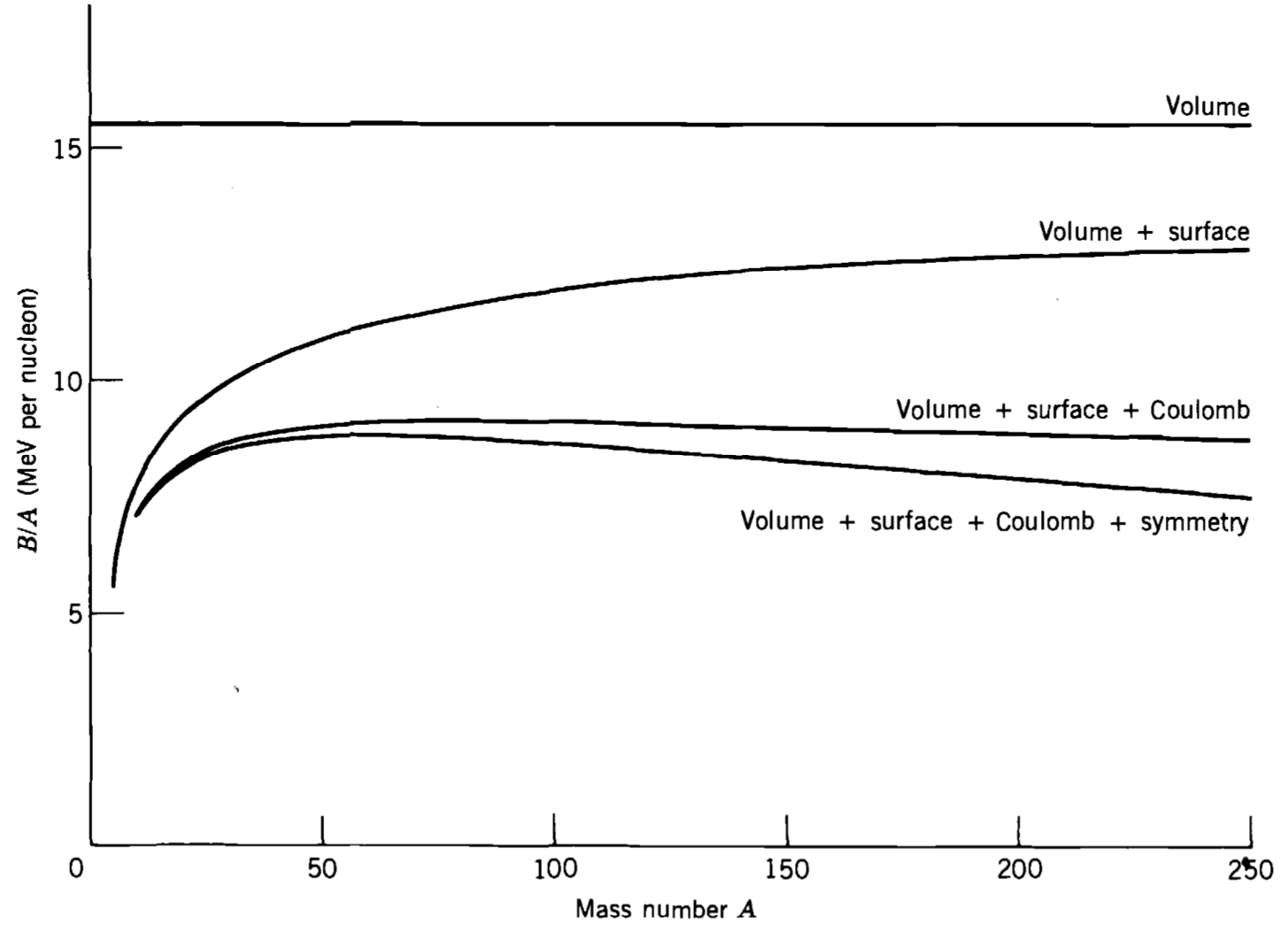
The volume term reflects the observation that \(B/A\) is approximately constant for medium and heavy nuclei. It is illuminating that this term is proportional to \(A\), rather than \(A(A-1)\).
A dependence on \(A(A-1)\) would suggest that every nucleon interacts strongly with every other nucleon. The observed dependence on \(A\) instead tells us that nucleons mainly interact with a limited number of nearby neighbours. This is another expression of the short-range, saturated nature of the nuclear force.
14.4.2 Surface Term
Nucleons at the nuclear surface have fewer neighbouring nucleons than those in the interior. They therefore experience less attractive nuclear force.
The volume term overestimates the binding of these surface nucleons. The surface term compensates for this by subtracting an amount proportional to the surface area:
The negative sign indicates that this is a destabilising contribution.
14.4.3 Coulomb Term
This term accounts for the destabilising Coulomb repulsion between protons. If we approximate the nucleus as a uniformly charged sphere, the electrostatic energy needed to assemble a charge \(Q=Ze\) into a sphere of radius \(R\) is
\[ E_C = \frac{3}{5} \frac{1}{4\pi\epsilon_0} \frac{(Ze)^2}{R}. \tag{14.9}\]
Since the nuclear radius satisfies \(R\propto A^{1/3}\), this suggests a Coulomb energy proportional to
\[ \frac{Z^2}{A^{1/3}}. \]
Since each proton sees every other proton there are \(Z(Z - 1)/2\) interactions. So, the SEMF uses \(Z(Z-1)\) instead of \(Z^2\). Thus, the Coulomb term has the form
\[ -\ac Z(Z-1)A^{-1/3}. \]
14.4.4 Symmetry Term
To understand the symmetry term, first note that
\[ A-2Z=N-Z. \]
The symmetry term becomes increasingly negative as we move away from \(N=Z\). This agrees with the observation that light stable nuclei usually have approximately equal numbers of protons and neutrons.
The origin of this term can be understood using the Fermi Gas Model. If \(N\neq Z\), the more numerous species must fill higher momentum states because of the Pauli Exclusion Principle. This increases the total kinetic energy. In particular, Equation 13.20 gives
\[ \Delta E \propto \frac{(N-Z)^2}{A} = \frac{(A-2Z)^2}{A}. \tag{14.10}\]
The symmetry term therefore discourages a very large neutron–proton imbalance. It helps explain why light nuclei with a very large neutron excess are unstable.
For heavy nuclei, the Coulomb repulsion between protons becomes increasingly important. The stable neutron-to-proton ratio is then determined by a competition between the Coulomb term, which favours fewer protons, and the symmetry term, which favours \(N\approx Z\).
14.4.5 Pairing Term
The table below shows trends observed in stable nuclei.
| Z | N | Number of Stable Nuclei |
|---|---|---|
| Even | Even | 165 |
| Even | Odd | 55 |
| Odd | Even | 50 |
| Odd | Odd | 4 |
The pairing term incorporates these observations by making even-even nuclei more stable and odd-odd nuclei less stable. The \(A^{-3/4}\) dependence is an empirically determined power law; some versions of the SEMF use \(A^{-1/2}\) instead.
14.4.6 Effect of the Various Terms
The figure below shows the relative effect of the various terms in the SEMF.
14.5 Mass Chains
The SEMF is useful for understanding general trends in stable nuclei. One important application is the study of mass chains.
A mass chain consists of isobars: nuclides with the same mass number \(A\). Consider the following table.
| Nuclide | \(A\) | Atomic Mass (amu) |
|---|---|---|
| \(\ele{In}{49}{125}{76}\) | \(125\) | \(124.9136738\) |
| \(\ele{Sn}{50}{125}{75}\) | \(125\) | \(124.9077894\) |
| \(\ele{Sb}{51}{125}{74}\) | \(125\) | \(124.9052543\) |
| \(\ele{Te}{52}{125}{73}\) | \(125\) | \(124.9044312\) |
Although all nuclei in a mass chain have the same \(A\), they do not have the same mass. Some are more stable than others. Less stable nuclei can move towards stability by converting a neutron into a proton through \(\beta^-\) decay, or by converting a proton into a neutron through \(\beta^+\) decay or electron capture.
The SEMF allows us to predict the \(\beta\)-stability of a mass chain.
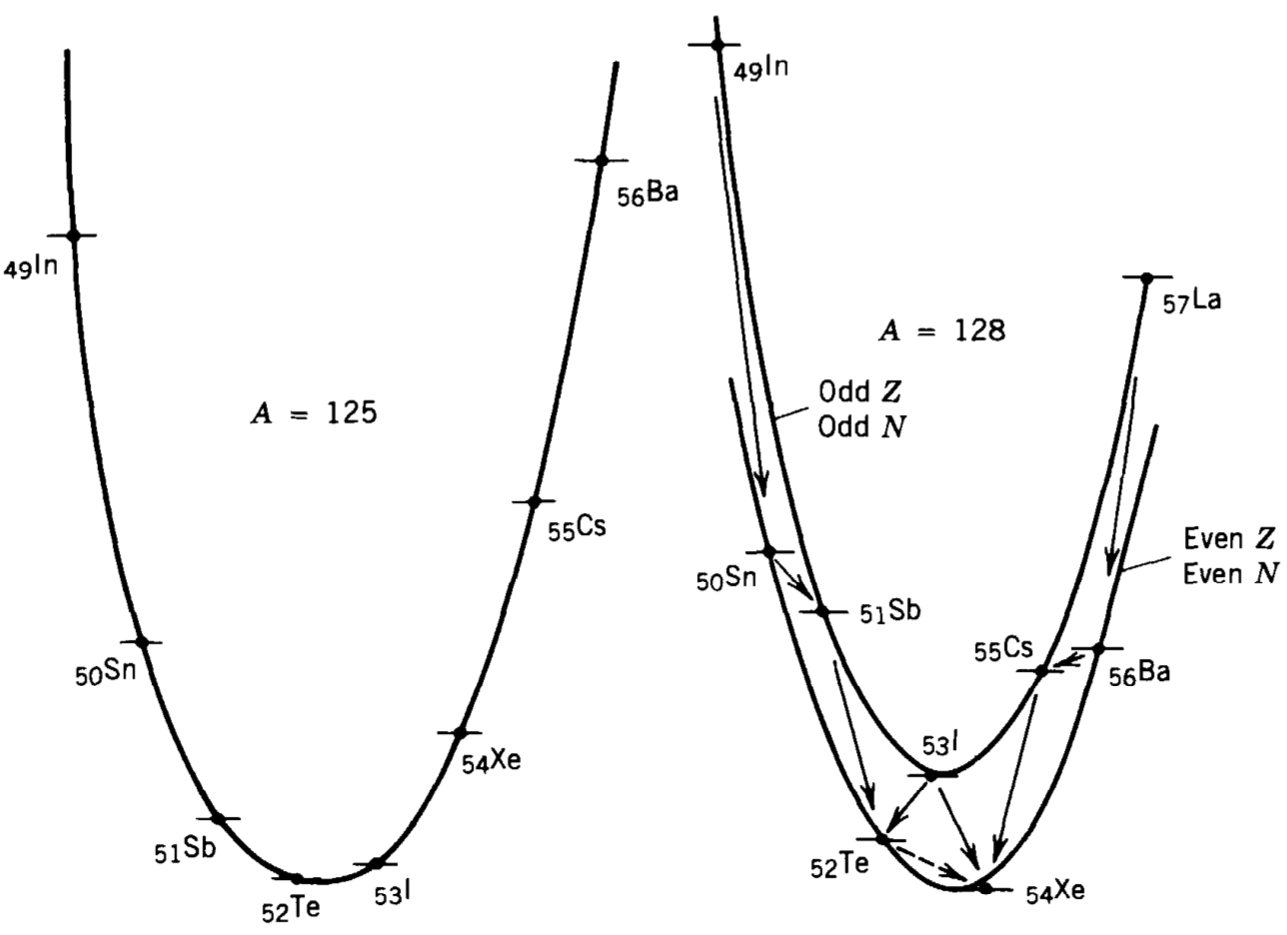
If we hold \(A\) constant, the semi-empirical mass formula, Equation 14.7, gives the atomic mass as a function of \(Z\). The resulting expression is quadratic in \(Z\). Thus, a plot of atomic mass \(M\) against \(Z\) has a parabolic shape.
The figure shows the resulting mass parabolas for \(A=125\) and \(A=128\). For odd \(A\), there is one parabola. For even \(A\), the pairing term produces two nearby parabolas: one for even-even nuclei and one for odd-odd nuclei.
The nucleus at the bottom of a mass parabola is the most stable isobar. For example, the mass chain with \(A=125\) has its stable nucleus near \(Z=52\). Unstable nuclei move towards this minimum through \(\beta^-\) decay, \(\beta^+\) decay, or electron capture. Double-\(\beta\) decay is also possible in some cases, but it is rare.
We can put this discussion into more mathematical terms. The most stable nucleus in a mass chain is found by minimising the mass energy with respect to \(Z\) while holding \(A\) fixed:
\[ \left( \frac{\partial M}{\partial Z} \right)_A = 0. \tag{14.11}\]
Using Equation 14.6 and Equation 14.7 gives
\[ Z_{\text{min}} = \frac{ m_n-M({}^1_1\mathrm H) + \ac A^{-1/3} + 4\ad }{ 2\ac A^{-1/3} + 8\ad A^{-1} }. \tag{14.12}\]
Since \(\ac\approx0.72\,\mathrm{MeV}\) and \(\ad\approx23\,\mathrm{MeV}\), the first three terms in the numerator are usually small compared with \(4\ad\). We may therefore write approximately
\[ Z_{\text{min}} \approx \left( \frac{A}{2} \right) \frac{1}{ 1+\dfrac{\ac}{4\ad}A^{2/3} }. \tag{14.13}\]
This expression predicts that \(Z_{\text{min}}\approx A/2\) for light nuclei, while heavier stable nuclei have \(Z_{\text{min}}<A/2\). In other words, heavy stable nuclei require more neutrons than protons.