13 Modelling the Nucleus I: Fermi Gas Model
\[ \newcommand\v[1]{\boldsymbol{#1}} \newcommand\vdot[2]{\v{#1}\cdot\v{#2}} \]
\[ \newcommand{\dd}[2][]{\mathrm{d}^{#1}#2} \]
\[ \newcommand\f[2]{\dfrac{#1}{#2}} \newcommand\da[2]{\dfrac{d #1}{d #2}} \newcommand\daa[2]{\dfrac{d^2 #1}{d #2^2}} \newcommand\pa[2]{\dfrac{\partial #1}{\partial #2}} \newcommand\pal[3]{\left.\dfrac{\partial #1}{\partial #2}\right|_{#3}} \newcommand\paa[2]{\dfrac{\partial^2 #1}{\partial #2^2}} \newcommand\pab[3]{\dfrac{\partial^2 #1}{\partial #2 \partial #3}} \def\half{\frac{1}{2}} \]
\[ \newcommand\ket[1]{\left|#1\right\rangle} % |x> \newcommand\exp[1]{\left\langle#1\right\rangle} % <x> \newcommand\lr[1]{\left(#1\right)} % (x) \newcommand\lrs[1]{\left[#1\right]} % [x] \newcommand\lra[1]{\left|#1\right|} % |x| \newcommand\lrc[1]{\left\{#1\right\}} % {x} \newcommand\lrl[3]{\left.#1\right|_{#2}^{#3}} % x_limits \]
\[ \def\ie{\text{i.e.}\quad} \]
\[ \newcommand{\me}[3][\rightarrow]{{#2}#1{#3}} % Typical reaction \newcommand{\nr}[3]{{#1}\,({#2})\,{#3}} % Nuclear reactions \newcommand{\ele}[4]{_{#2}^{#3}{\textbf{#1}}_{#4}} \newcommand{\el}[2]{^{#2}\text{#1}} \newcommand{\til}[2][\mathbf{\sim}]{\underset{#1}{{#2}}} \newcommand{\b}[1]{\overline{#1}} \]
\[ \newcommand{\coulomb}[1]{\dfrac{#1}{4\pi\epsilon_0}} \def\degree{^*} \]
\[ \def\amu{\text{ amu}} \def\J{\text{ J}} \def\K{\text{ K}} \def\s{\text{ s}} \def\second{\text{ s}} \def\Psecond{\text{ s}^{-1}} \def\m{\text{ m}} \def\mm{\text{ mm}} \def\km{\text{ km}} \def\fm{\text{ fm}} \def\mum{\text{ $\mu$m}} \def\mus{\text{ $\mu$s}} \def\mPERs{\text{ ms$^{-1}$}} \def\eV{\text{ eV}} \def\keV{\text{ keV}} \def\GeV{\text{ GeV}} \def\MeV{\text{ MeV}} \def\MeVc{\text{ MeV/c$^2$}} \def\KeVc{\text{ KeV/c$^2$}} \newcommand\ttp[1]{\times 10^{#1}} % To The Power \]
\[ \def\en{\nu_e} \def\Aen{\b{\nu_e}} \def\mun{\nu_\mu} \def\Amun{\b{\nu}_\mu} \]
\[ \def\uraniumA{\ele{U}{92}{233}{}} \def\uraniumB{\ele{U}{92}{235}{}} \def\uraniumC{\ele{U}{92}{238}{}} \def\carbonB{\ele{C}{6}{14}{}} \def\nitrogenB{\ele{N}{7}{14}{}} \def\oxygenA{\ele{O}{8}{14}{}} \def\oxygenB{\ele{O}{8}{16}{}} \]
\[ % \def\com{\text{\scriptsize CM}} \def\com{\mathrm{\scriptsize CM}} \]
\[ \def\l{l} \]
\[ \def\g{\gamma} \]
What To Expect In This Chapter
Following Rutherford’s work establishing the existence of the nucleus, there was a need to understand how nuclei are structured and to explain observed features such as binding energy and the preferred neutron-to-proton ratio.
In this chapter, we will develop a simple model for the nucleus called the Fermi Gas Model. This model will help us understand how the \(N/Z\) ratio affects the energy and stability of a nucleus. It will also be useful later when we develop a theoretical understanding of nuclear binding energy.
13.1 A Word About Theoretical Models
Models are one of our strategies for understanding the various phenomena in our Universe. It is good to be clear about our expectations of a model, so allow me first to speak about the idea, or spirit, of a model.
Sometimes, a simple and mathematically tractable theory that gives physical insight and makes predictions is more valuable than a model that attempts to include every detail but is impossible to use. If a simple model does not describe experiments perfectly, we can identify what it misses and introduce an appropriate correction. Most models in physics, especially in nuclear physics, follow this spirit.
13.2 Modelling The Nuclear Force
13.3 Modelling The Nuclear Force
First, it is important to distinguish between the strong interaction between quarks and the nuclear force between nucleons. Quantum Chromodynamics (QCD) describes the interaction between quarks and gluons. The nuclear force is the residual effect of this interaction that acts between protons and neutrons, rather like the residual electromagnetic interaction that allows electrically neutral atoms to attract one another.
Our fundamental understanding of the strong interaction therefore comes from QCD. However, a direct QCD description of an entire nucleus is too sophisticated for our present purposes. Instead, it is more instructive to take a step back and see how early nuclear models were developed.
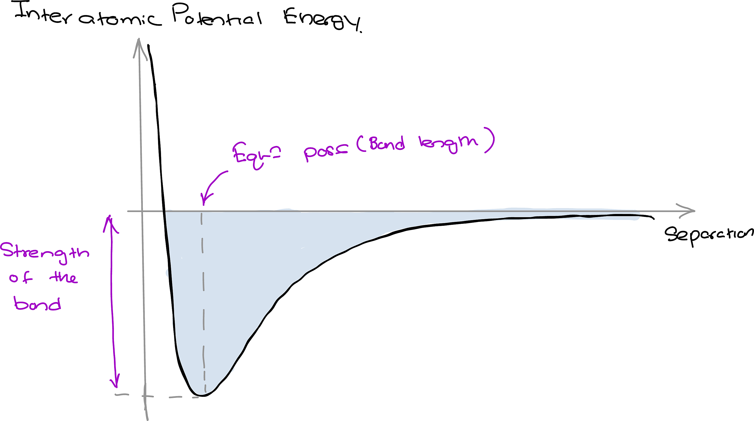
We know that the nuclear force is attractive over distances of roughly a few femtometres. However, it must also become repulsive at very short internucleon distances; otherwise, the nucleons would collapse into the same region.
This is reminiscent of our understanding of intermolecular forces, which motivates phenomenological models such as the Lennard–Jones potential shown in the upper panel of Figure 13.1. Building on this idea, and keeping in mind that “cows are really spheres,” we can model the nuclear force using the square-well potential shown in the lower panel.
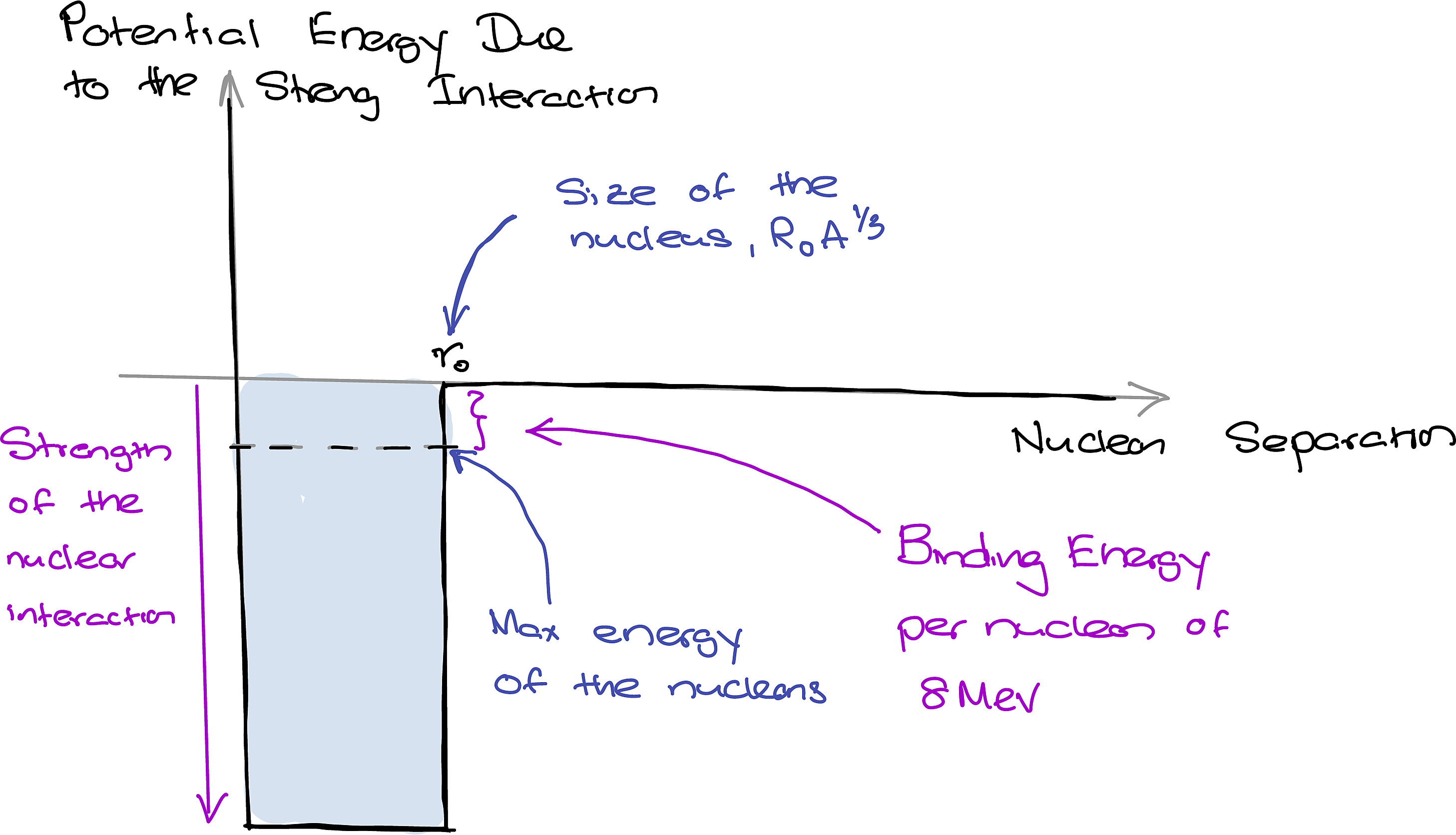
This model is certainly crude, but it is mathematically tractable and physically intuitive. We can use it to develop a model of the nucleus known as the Fermi Gas Model. While its numerical predictions will not be exact, the insights it gives us are invaluable.
Before moving on, let me highlight two details of the square-well model:
- The depth of the well indicates the strength of the attractive nuclear interaction. Compare this with the ground-state energy of hydrogen, which is \(-13.6\,\mathrm{eV}\).
- A nucleon near the top of the occupied levels must still require roughly \(8\,\mathrm{MeV}\) to be removed from a typical nucleus. This gives us a useful order-of-magnitude estimate of the depth of the top of the well.
13.4 Setting Up The Fermi Gas Model
Let us now consider the assumptions and features of the Fermi Gas Model of the nucleus.
13.4.1 The Nucleons Live In A Square Well
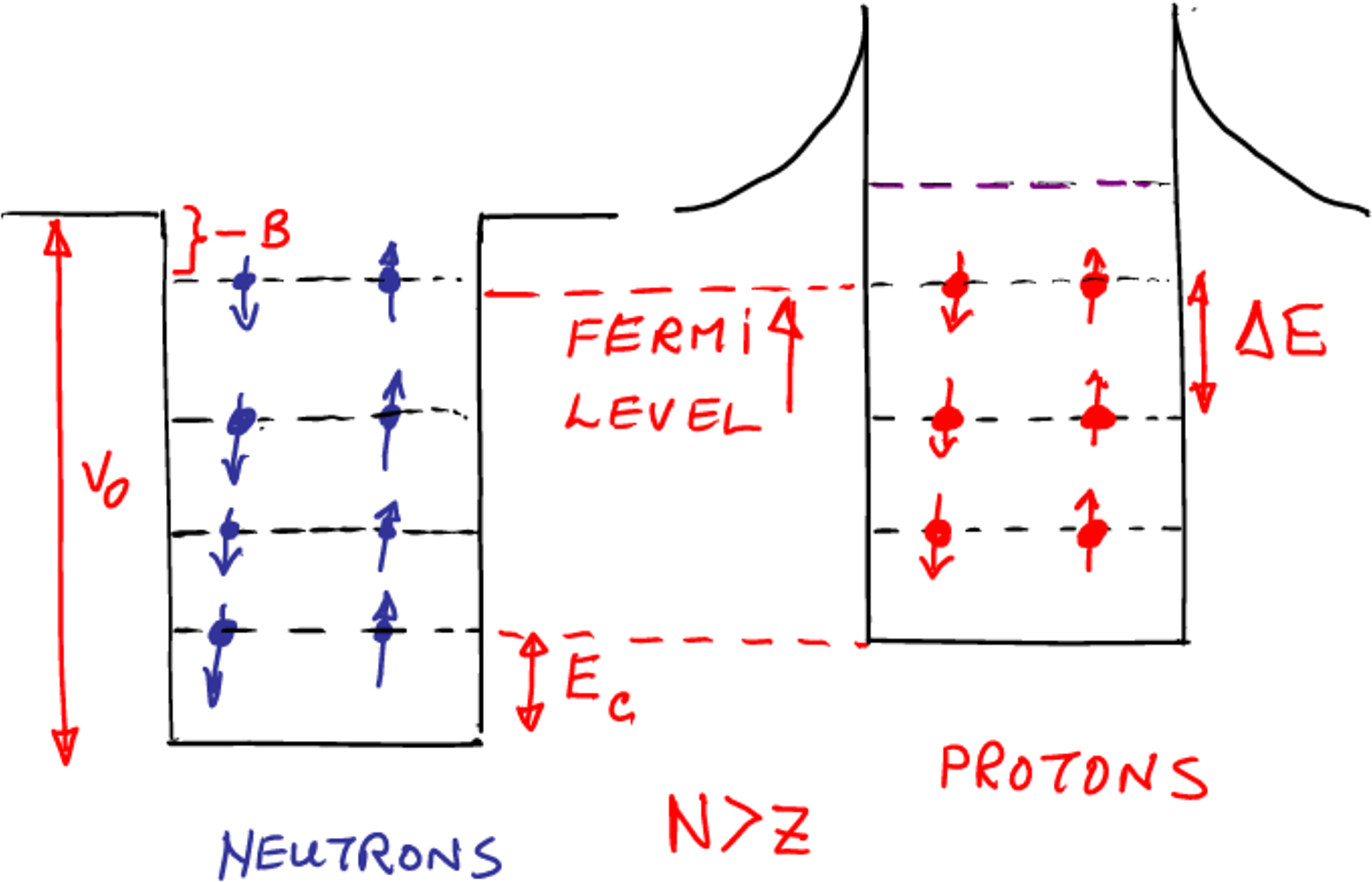
In the Fermi Gas Model, protons and neutrons move independently in the average, or mean, field created by all the other nucleons. Based on our discussion above, we approximate this field using a three-dimensional square well.
13.4.2 The Proton Well Has A Coulomb ‘Skirt’
Unlike neutrons, protons experience Coulomb repulsion in addition to the strong interaction. Thus, outside the nuclear well, the proton potential differs from the neutron potential. This is shown in Figure 13.2, where the proton well has a Coulomb “skirt”.
Furthermore, since protons and neutrons are fermions, the Pauli Exclusion Principle restricts how they can occupy the available states. Each spatial state can contain at most two nucleons of a given type: one with spin up and one with spin down.
13.4.3 The Two Systems Must Have A Common Fermi Level
The maximum occupied energies of the proton and neutron systems, called their Fermi energies, must be the same:
\[ E_{F,n}=E_{F,p}. \tag{13.1}\]
Although the proton and neutron systems contain different numbers of particles, their highest occupied states must lie at the same energy.
There are two arguments to support this requirement:
- It is experimentally observed that the energy required to liberate a nucleon is the same, regardless of whether it is a proton or a neutron.
- If \(E_{F,n} \gt E_{F,p}\), for nuclei with \(N>Z\), neutrons will find it energetically favourable to turn into a proton via \(\beta\)-decay. So, all nuclei with \(N>Z\) should be unstable, which is not true. The \(N/Z\) ratio is on average about \(1.58\) (about 60:40) for stable, high \(Z\) nuclear.
13.4.4 Different Potential-Well Depths for Neutrons and Protons
A consequence of insisting that the proton and neutron Fermi energies are the same is that the bottoms of their potential wells must differ. This is inevitable because, typically, \(N\neq Z\). The two types of nucleon therefore fill different numbers of available fermion states and have different kinetic Fermi energies. Shifting the well bottoms compensates for this difference and allows the highest occupied proton and neutron states to have the same Fermi energy.
13.5 Depth Of The Potential Well
Let us now make the discussion more quantitative. First, we estimate the Fermi energies of the protons and neutrons.
Recall that the Schrödinger equation for a particle in a three-dimensional box of side \(L\) gives quantised energies of the form
\[ E_{n_x,n_y,n_z} = \frac{\hbar^2\pi^2}{2mL^2} \left( n_x^2+n_y^2+n_z^2 \right), \tag{13.2}\]
where \(n_x\), \(n_y\), and \(n_z\) are positive integers.
Let \(n_F\) correspond to the highest occupied level such that:
\[ n_F^2=n_x^2+n_y^2+n_z^2. \tag{13.3}\]
with corresponding kinetic Fermi energy:
\[ E_F = \frac{\hbar^2\pi^2}{2mL^2}n_F^2, \tag{13.4}\]
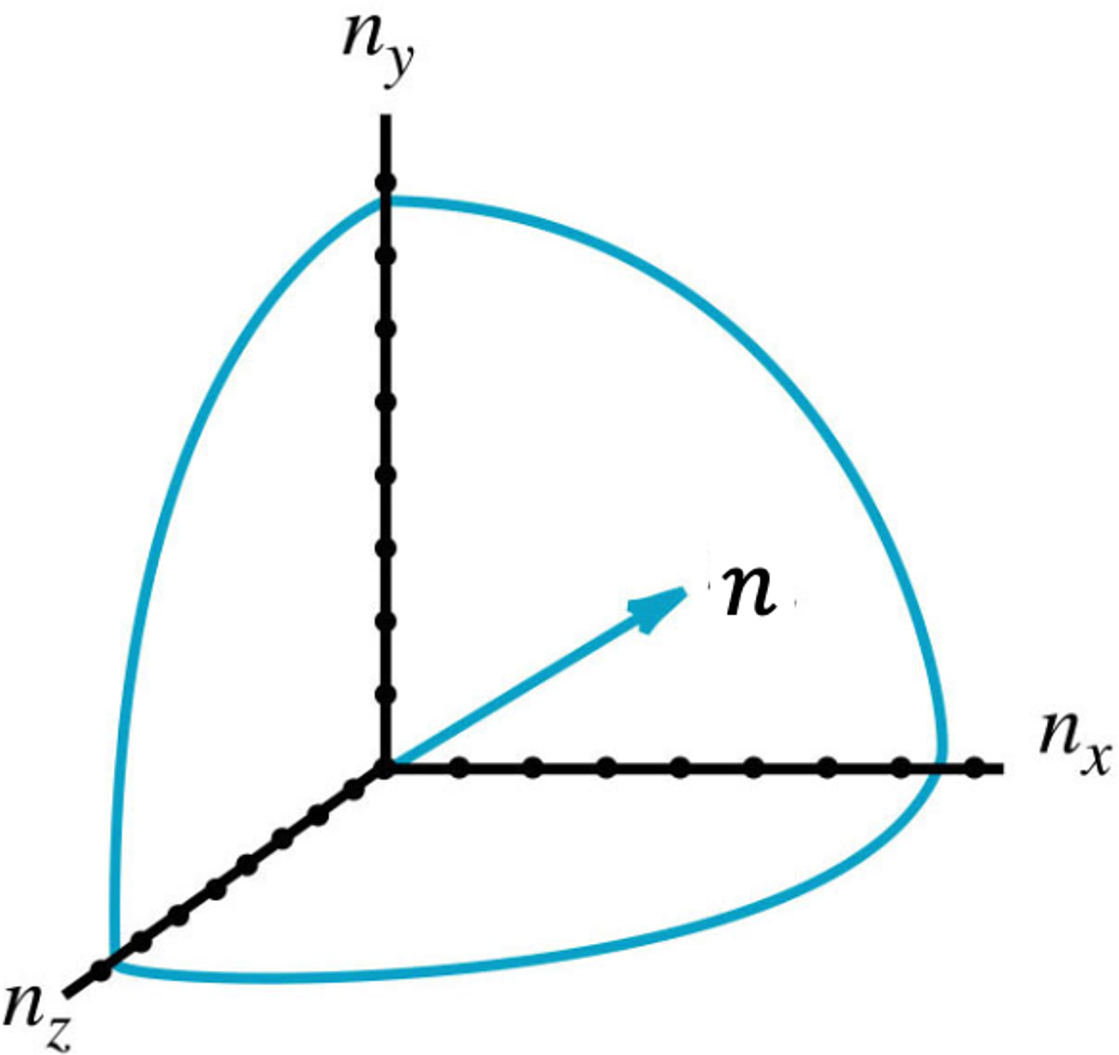
Suppose the boxes contains \(\mathcal N\) particles. All allowed states must lie in the positive octant of a sphere of radius \(n_F\), as shown in Figure 13.3. Thus,
\[ \mathcal N = \left( \frac{1}{8}\times\frac{4}{3}\pi n_F^3 \right) \times2 = \frac{\pi}{3}n_F^3. \tag{13.5}\]
The factor of \(2\) accounts for the two possible spin states of a spin-\(\tfrac12\) fermion.
Combining Equation 13.4 and Equation 13.5 gives
\[ E_F = \frac{\hbar^2}{2m} \left( \frac{3\pi^2\mathcal N}{L^3} \right)^{2/3}. \tag{13.6}\]
Let us now adapt Equation 13.6 to the nucleus. Since \(L^3\) is the volume of the box, we replace it using the empirical nuclear-radius formula:
\[ L^3 \rightarrow \frac{4}{3}\pi(R_0A^{1/3})^3 = \left( \frac{4\pi R_0^3}{3} \right)A. \tag{13.7}\]
We then obtain
\[ E_F = \frac{\hbar^2}{2mR_0^2} \left( \frac{9\pi}{4} \right)^{2/3} \left( \frac{\mathcal N}{A} \right)^{2/3}. \tag{13.8}\]
If we define
\[ f=\frac{\mathcal N}{A}, \tag{13.9}\]
then
\[ E_F = \frac{\hbar^2}{2mR_0^2} \left( \frac{9\pi}{4} \right)^{2/3} f^{2/3}. \tag{13.10}\]
For a representative heavy stable nucleus, we may take approximately \(N/A\approx0.60\) and \(Z/A\approx0.40\). This gives the kinetic Fermi energies
\[ E_F \approx \begin{cases} 28.8\,\mathrm{MeV} & \text{(protons)},\\ 37.7\,\mathrm{MeV} & \text{(neutrons)}. \end{cases} \tag{13.11}\]
A nucleon near the Fermi level requires approximately \(8\,\mathrm{MeV}\) to be removed. Thus, as a rough estimate, the well depths must be of order
\[ \text{well depth} \approx \begin{cases} 28.8+8\approx37\,\mathrm{MeV} & \text{(protons)},\\ 37.7+8\approx46\,\mathrm{MeV} & \text{(neutrons)}. \end{cases} \tag{13.12}\]
These values are only estimates; they depend on the chosen values of \(N/A\) and \(Z/A\).
13.6 Density Of States
If we can determine the energy associated with a particular \(N-Z\) configuration, then we can ask which configuration minimises the energy and is therefore most stable. For this, we need to know how nucleons are distributed among the available energy levels. This is described by the density of states, \(D(E)\).
The density of states is defined so that \(D(E)\,dE\) gives the number of available states between \(E\) and \(E+dE\).
From Equation 13.5,
\[ \mathcal N = \frac{\pi}{3}n^3. \]
Therefore,
\[ d\mathcal N = \pi n^2\,dn. \tag{13.13}\]
Using Equation 13.2, write
\[ E_n = \frac{\hbar^2\pi^2}{2mL^2}n^2 = \Theta n^2, \tag{13.14}\]
where \(\Theta\) is introduced temporarily for convenience. Differentiating gives
\[ \frac{dE_n}{dn} = 2\Theta n = 2\sqrt{\Theta E_n}. \tag{13.15}\]
Thus,
\[ \begin{aligned} d\mathcal N &= \pi n^2\,dn \\ &= \pi \left( \frac{E_n}{\Theta} \right) \frac{dE_n}{2\sqrt{\Theta E_n}}, \end{aligned} \]
and hence
\[ D(E) = \frac{d\mathcal N}{dE} = \frac{\pi}{2\Theta^{3/2}}E^{1/2}. \tag{13.16}\]
Substituting for \(\Theta\) gives
\[ D(E) = \frac{(2m)^{3/2}L^3}{2\pi^2\hbar^3} E^{1/2}. \tag{13.17}\]
The density of states increases with energy. There are therefore more available states at higher energies than at lower energies.
13.7 Total Energy Of The Nucleons
\[ \newcommand\t[1]{\int_0^{E_F}{#1}\,D(E)dE} \]
Now, let’s calculate the total average energy of the nucleons. For, this, we need to evaluate the following for both neutrons and protons.
\[ \exp{E} = \f{\displaystyle \t{E}}{\displaystyle \t{}} \tag{13.18}\]
Using this along with ?eq-ferm-energy-2 gives us that:
\[ \exp{E_\text{Total}} \approx \f{3}{10m}\f{\hbar^2}{R_0^2}\lr{\f{9\pi}{4}}^{2/3}\lr{\f{Z^{5/3}+N^{5/3}}{A^{2/3}}} \tag{13.19}\]
This result has an important consequence. For fixed \(A=N+Z\), the kinetic energy is smallest (see the supplementary questions) and the system most most stable when \(N=Z\).
Any difference between \(N\) and \(Z\) forces one species to occupy more high-energy states than the other. This increases the total kinetic energy because of the Pauli Exclusion Principle. This instability of energy \(\Delta E\) (from the most stable configuration) is given by:
\[ \Delta E \approx \f{1}{3m}\f{\hbar^2}{R_0^2}\lr{\f{9\pi}{2^{6}}}^{2/3} \f{\delta^2}{A} \propto \f{(A-2Z)^2}{A} \tag{13.20}\]
Where \(\delta=N-Z\) gives the number of excess neutrons.