1 Particle Physics: A Summary

1.1 What To Expect In This Chapter

Particle Physics can be described as the ongoing effort to answer the question, “What is matter?” It is certainly not a new question. People have been trying to answer this for thousands of years. There was a time when the answer involved ‘basic elements’ like Earth, Fire, Water, and Air. The more modern answer to this question is (unimaginatively) named the Standard Model of Physics. In this chapter, I will quickly give you the gist of the Standard Model. This will provide a broad appreciation of the Standard Model while building our foundation for the discussions in the following chapters.

1.2 The Standard Model: The Good, The Bad And The Ugly

1.2.1 The Good

You can think of the Standard Model as a relativistically correct quantum theory. The Standard Model is enviable in its ability to predict. For example, the Higgs boson was predicted about 50 years before it was discovered at CERN, in 2012. Even more impressive (at least for me) is that it can predict values with mind-boggling accuracy. For example, consider \(g_e\), the factor that connects the electron’s spin angular momentum, \(\v{s}\) and its magnetic dipole moment \(\v{\mu}_e\): \[ \v{\mu_e} = g_e \lr{\f{e}{2m_e}}\v{s} \tag{1.1}\]

Here is the comparison between the theoretical and experimental values:

Theory	2.002 319 304 36
Experiment	2.002 319 304 362 56(35)

Table 1.1: An example of the agreement between a Standard Model prediction and experiment.

1.2.2 The Bad And The Ugly

The Standard Model has several areas for improvement. For one, it requires many experimental parameters (such as the masses of the elementary particles) to be supplied as inputs, when we would really like the theory itself to predict them. Furthermore, its predictions are not always spectacular. For example, the theoretical value of the proton mass is still about 3% away from the measured value!

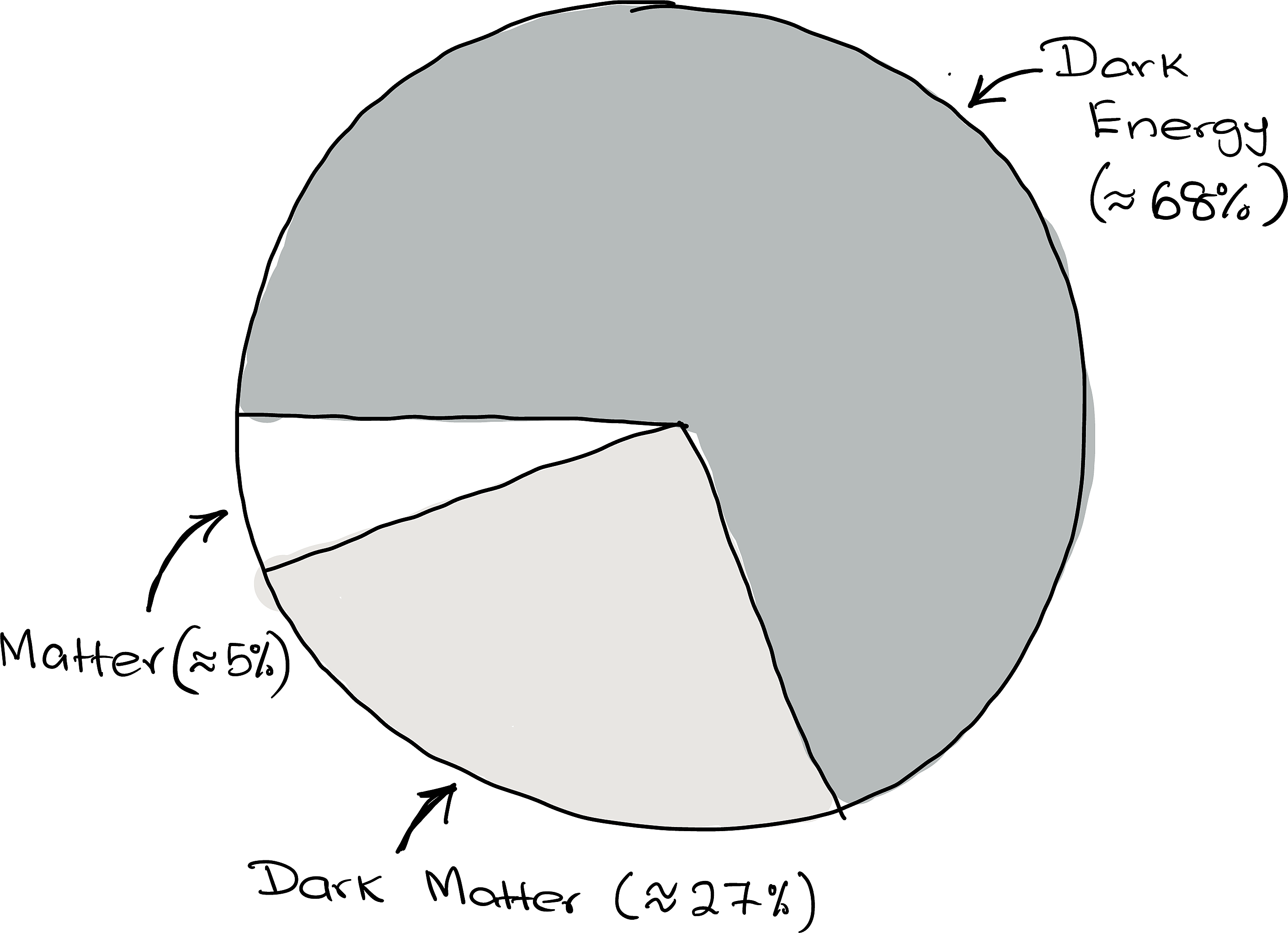
The Standard Model also cannot incorporate gravity. Most glaringly, it accounts for only about 5% of the observed Universe; the rest consists of dark matter and dark energy.

Figure 1.1: The Standard Model can account for only 3% of the mass of the Universe.

1.2.3 The Standard Model In A Nutshell

Quick reminder

Fermions

Fermions are particles with half-integer spin (e.g. \(\frac{1}{2}\hbar,\frac{3}{2}\hbar,\ldots\))
Fermions are described by Fermi-Dirac statistics.
Fermions have antisymmetric wavefunctions.
I.e. under an exchange of identical fermions \(\psi \rightarrow -\psi\).

Bosons

Bosons are particles with integer spin (e.g. \(\hbar,2\hbar,\ldots\))
Bosons are described by Bose-Einstein statistics.
Bosons have symmetric wavefunctions.
I.e. under an exchange of identical bosons \(\psi \rightarrow \psi\).

Let me start by painting you a simplified picture of The Standard Model that includes all the essentials. We can then incrementally improve on it. So, here goes…

The Universe works due to the collective effort of the following:

Ingredient 1: 12* Elementary Fermions

All matter is ultimately made up of just 12 fundamental fermions and their 12 anti-particles (hence the asterisk).

Ingredient 2: Four Interactions

These fundamental particles interact with each other via four fundamental interactions:

Gravity,
Electromagnetic(EM),
Weak,
Strong.

Ingredient 3: Symmetries

These interactions are constrained by the various symmetries of our Universe (e.g., translational symmetry).
These constraints manifest as conservation laws (e.g., conservation of momentum).

I hope you realise how absurdly simple this sounds. Well, it is … sort of.

1.3 Ingredient 1: Interactions

1.3.1 The Importance of Interactions

All four interactions are essential to keeping our Universe working as we observe it. The gravitational interaction is the weakest, yet it shapes the large-scale structure of the Universe. The electromagnetic (EM) interaction, together with quantum mechanics, arranges electrons and nuclei into atoms. The strong interaction binds protons and neutrons within the nucleus at the atom’s core. The weak interaction allows nuclei to transform and makes processes such as fusion in the Sun possible. It is also exceptional in violating parity conservation (more about that later).

In this section, let us examine how the Standard Model describes and incorporates interactions.

1.3.2 Quantum Fields & Virtual Particles

Before proceeding, we must update our picture of classical fields to one of quantum fields.

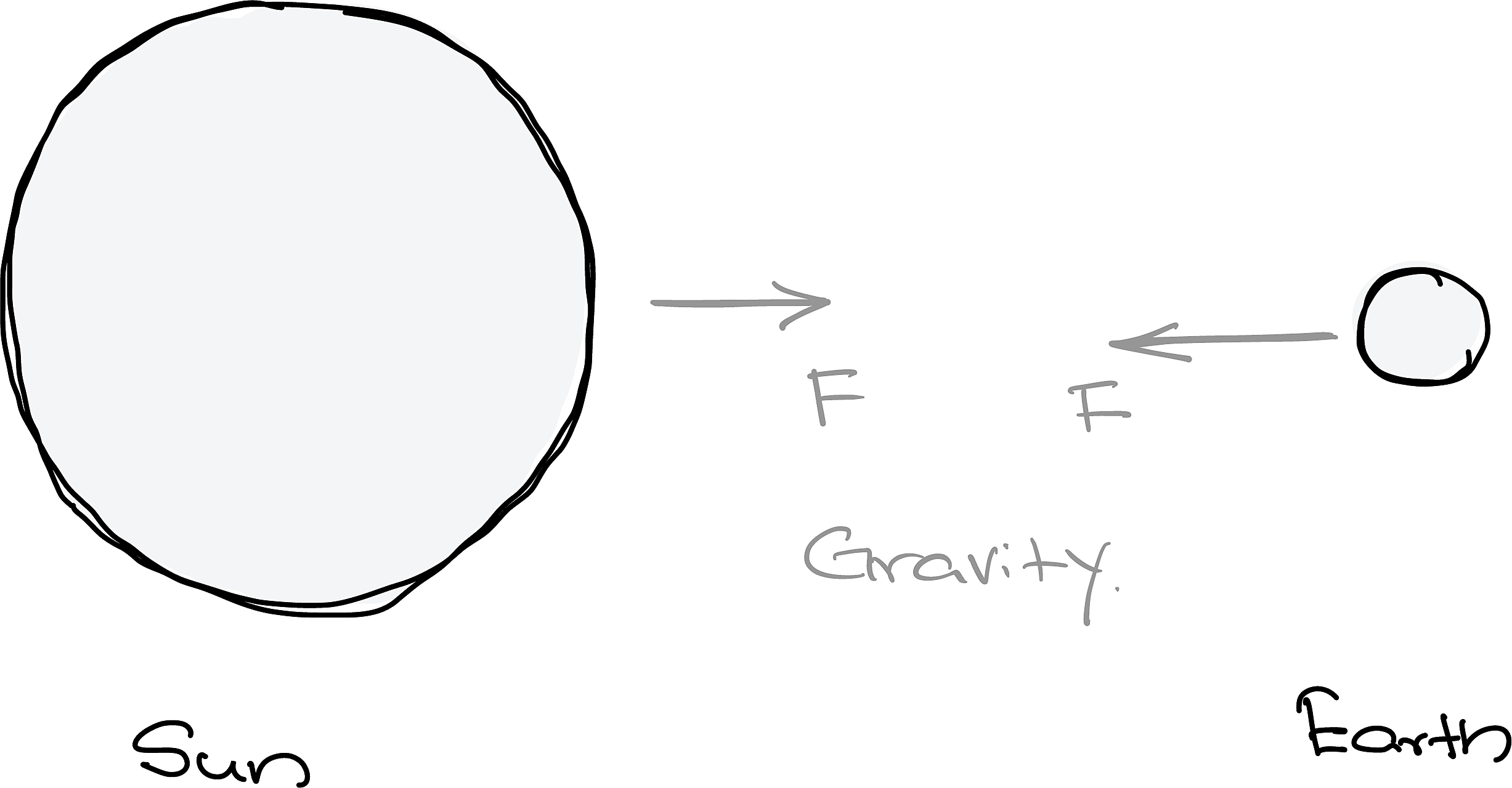
Let us begin with a simple(albeit fantastical) example. Consider the Sun–Earth system in Figure 1.2. What if something were to happen that made the Sun suddenly “disappear”? Yes, it is a little sci-fi, but play along. The important question is: when would the Earth know that something was wrong?

Newtonian gravity says “instantly”, but relativity does not permit information to travel faster than light! A more acceptable description therefore requires news of the Sun’s disappearance to propagate at a speed consistent with relativity.

Figure 1.2: A Gedankenexperiment to help us make sense of quantum fields.

In quantum field theories, interactions can be pictured as being mediated by virtual particles; force-carrying messenger particles exchanged between interacting objects. This picture also helps resolve the classical problem of “action at a distance”: momentum is no longer transferred across empty space without something mediating the interaction.The Standard Model incorporates five force-carrying virtual particles, all bosons (called gauge bosons).

Be very careful! The virtual particles that appear in calculations are not your run-of-the-mill particles. They are funky “versions” of real particles and cannot be observed directly. A virtual photon, for example, is not the same as the perfectly nice photon that has just entered your eye.

This exchange-particle picture emerges from quantum field theory (QFT). A proper discussion of QFT is way, way beyond the confines of this course (and possibly my neuronal capacity). However, I will come back to this briefly at the end of this chapter once we have discussed more about the Standard Model.

Before moving on, I should add that, despite the theory being more than 50 years old, there is still debate (e.g.,¹) over whether virtual particles should be regarded as physically real or merely as mathematical devices.

1.3.3 The Gauge Bosons of The Standard Model

Interaction	Particle	Spin	Mass	Charge	Relative Strength	Typical Timescale (s)	Range (m)	Typical cross section	Name of Theory	Other details
Strong	Gluon (\(g\))	1	0	0	1	\(10^{-23}\)	\(10^{-15}\)	\(10^{-30}\)	Chromodynamics	Yukawa (pions, 1934), Quantum Chromodynamics(QCD, 1970)
Weak	Vector Boson (\(W^{\pm1}, Z^0\))	1	80.433 GeV, 91.188 GeV	\(\pm1\) \(0\)	\(10^{-8}\)	\(10^{-8}\)	\(10^{-18}\)	\(10^{-44}\)	Flavordynamics	\(\beta\)-decay(1933), Electroweak(1960s)
EM	Photon (\(\gamma\))	1	0	0	\(10^{-3}\)	\(10^{-20}\)	\(\infty\)	\(10^{-33}\)	Electrodynamics	Maxwell(1865), Quantum Electrodynamic(QED, 1940s)
Gravity	Graviton (\(G\))	2	0	0	\(10^{-37}\)		\(\infty\)		Geometrodynamics	Newton(1679), General Relativity(1915)

Table 1.2: The Gauge Bosons (Force carriers) of the Standard Model.

Table 1.2 shows the five particles that mediate the four interactions. High-energy collisions between particles can produce real versions of these messenger particles. This is how we know experimentally that they exist. Also shown are some important “characteristics” of the fundamental interactions.

You can think of the cross-section as an indication of how readily an interaction occurs. For example, the strong interaction is not only strong but, when all else is equal, also the most likely of the three Standard Model interactions to occur. However, it has a minuscule range.

1.3.4 Picturing Interactions

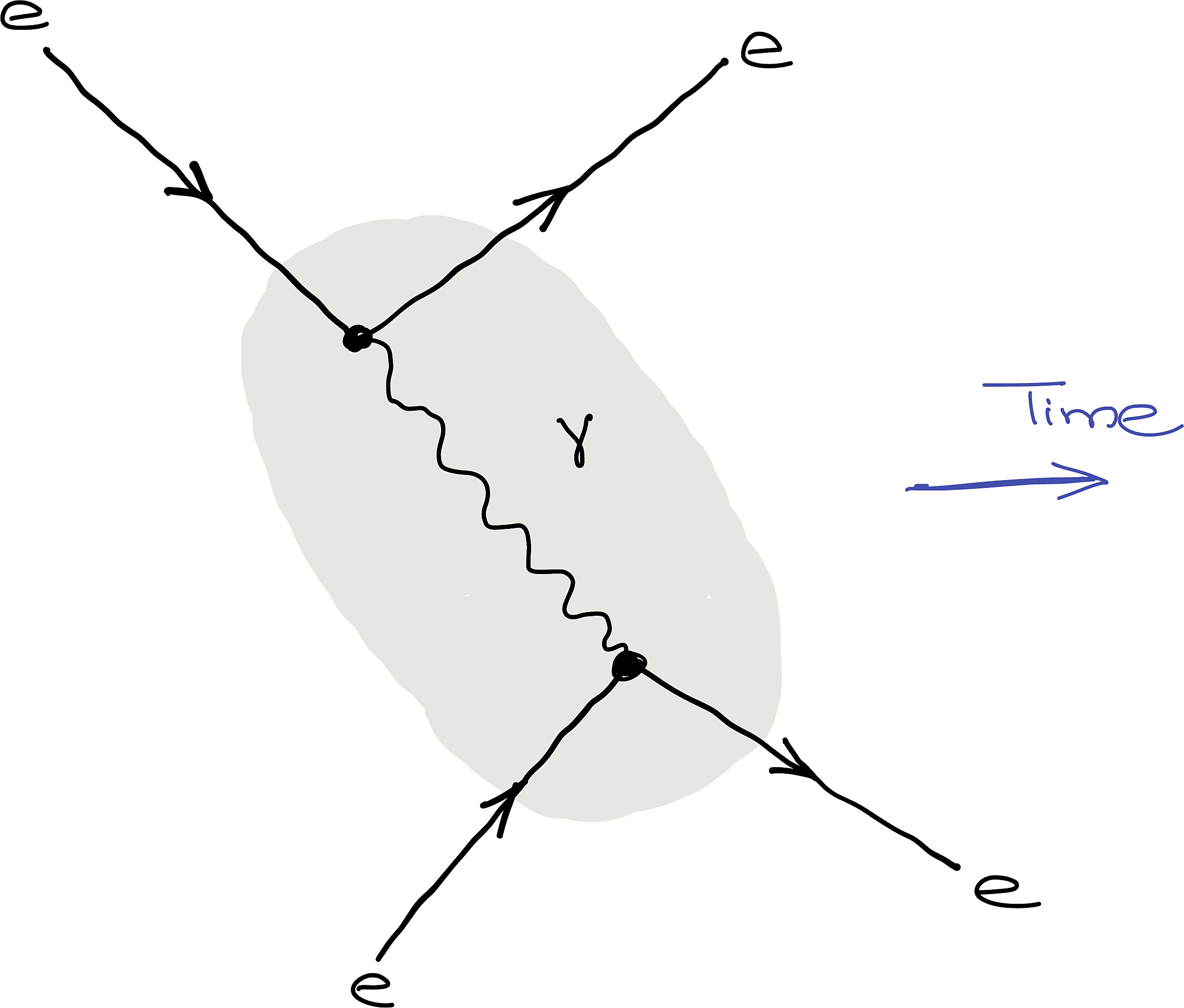
Figure 1.3: A way to picture how interactions occur.

Although I used the Sun–Earth system to introduce virtual particles, it is not the most suitable example because gravity is not part of the Standard Model. Let us therefore consider the more relevant example of an electron–electron interaction¹.

We can represent the electromagnetic interaction between two electrons “diagrammatically”, as shown in Figure 1.3. This is an example of a Feynman diagram. It depicts the two electrons interacting through the exchange of a mediating virtual photon.

Things to take note of:

Time flows from left to right: You can picture this by imagining a vertical line scanning across the diagram.
The lines are not trajectories. They simply indicate what enters and leaves the central interaction region.
The central region is never observed: The central region contains the inner workings of the interaction, in this case, the exchange of a virtual photon. What happens within this region is never observed directly.

Feynman diagrams are more than just pictures: they represent mathematical expressions that allow us to calculate the probability of an interaction. We will return to them later, although not at the mathematical level.

1.4 Ingredient 2: The Elementary Particles

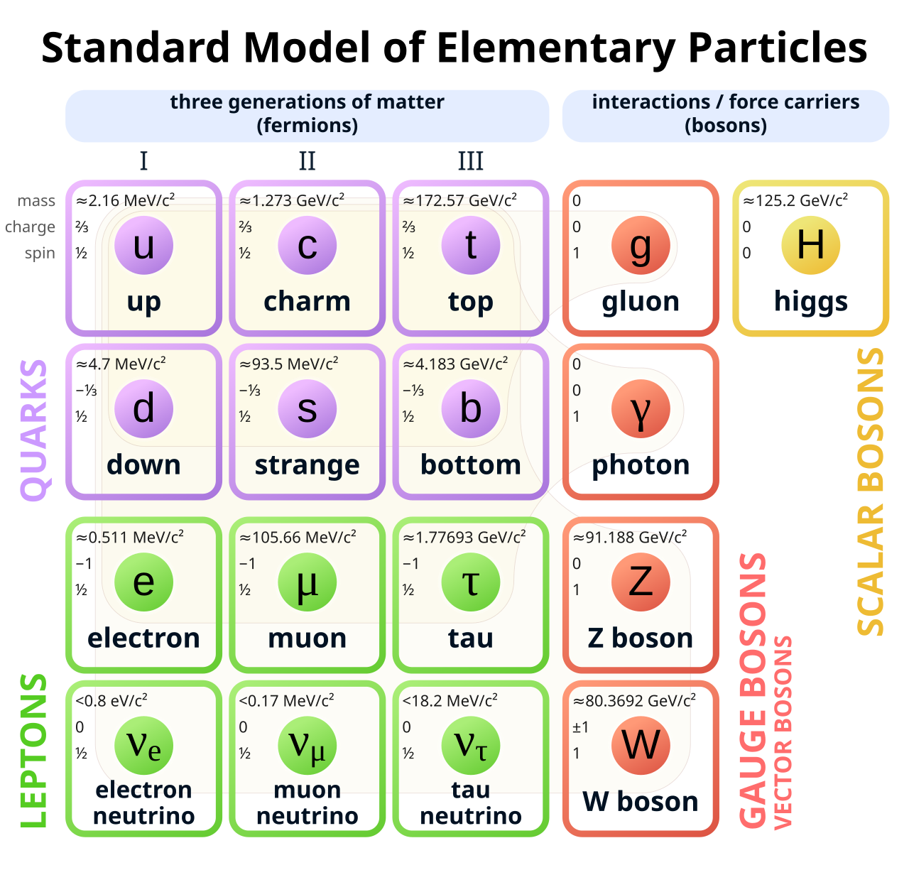
Figure 1.4: The elementary particles of the Standard Model. (Source: Wikipedia)

Now let’s focus on the elementary particles of the Standard Model. By the way, these particles are ‘elementary’ because they have no internal structure (as far as we know).

1.4.1 Particle Flavours

There are two families of elementary particles: leptons and quarks, with three generations each. All are fermions. A trend common to both families is that each generation is more massive than the previous one.

For the leptons, mass is the only difference between the generations. All the other interactions are identical. The neutrinos are not massless, but their masses are too small to be reliably measured with the techniques presently at our disposal.

We use the term flavour to distinguish the different members of each family. Thus, there are six flavours of quark and six flavours of lepton (all very yummy).

Generation	Particle	Symbol	Mass (MeV)	Charge
1	Electron	\(e^-\)	0.5	\(-1\)
	Electron neutrino	\(\nu_e\)	\(<10^{-6}\)	0
2	Muon	\(\mu^-\)	106	\(-1\)
	Muon neutrino	\(\nu_\mu\)	\(<10^{-6}\)	0
3	Tau	\(\tau^-\)	178	\(-1\)
	Tau neutrino	\(\nu_\tau\)	\(<10^{-6}\)	0

(a) The lepton family.

Generation	Particle	Symbol	Mass (MeV)	Charge
1	Down	\(d\)	3	\(-1/3\)
	Up	\(u\)	5	\(+2/3\)
2	Strange	\(s\)	1000	\(-1/3\)
	Charm	\(c\)	1300	\(+2/3\)
3	Bottom	\(b\)	4500	\(-1/3\)
	Top	\(t\)	174,000	\(+2/3\)

(b) The quark family.

Table 1.3: : Elementary particles come in six falvours of quarks and six flavours of leptons.

1.4.2 Elementary Particles, Interactions & Colour Charge

Family	Symbols	Strong	EM	Weak
Quarks (All)	\(d, u, s, c, b, t\)	Yes	Yes	Yes
Leptons (charged)	\(e^-, \mu^-, \tau^-\)	No	Yes	Yes
Leptons (neutrino)	\(\nu_e, \nu_\mu, \nu_\tau\)	No	No	Yes

Table 1.4: Do all particles participate in all the interactions?

Table 1.4 above shows whether each fundamental matter particle couples to the various fundamental interactions. Not every particle interacts through all four interactions.

You will notice that all the matter particles except neutrinos interact electromagnetically. Neutrinos carry no electric charge and hence do not “feel” the electromagnetic interaction.

Other types of charge determine whether a particle couples to the other interactions. For example, a particle must carry colour charge to feel the strong interaction. Quarks carry colour charge, whereas leptons do not. A quark’s colour may be red (R), green (G) or blue (B). Gluons also carry colour charge; in fact, each gluon corresponds to a quantum superposition of colour–anticolour combinations, such as \(C\bar{C}\).

And yes; you also need the appropriate “charge” to feel the weak interaction. All elementary fermions participate in the weak interaction.

1.4.3 Labels!

Elementary particles also possess other properties—for example, the strangeness of strange quarks and the charm of charm quarks. We therefore need additional labels, or quantum numbers, to describe them. We will discuss where these quantum numbers come from in the next chapter. For now, let us simply get comfortable using them.

Here is a list of the relevant quantum numbers:

Quantum number	Symbol	Applies to
Electron lepton number	\(L_e\)	First-generation leptons.
Muon lepton number	\(L_\mu\)	Second-generation leptons.
Tau lepton number	\(L_\tau\)	Third-generation leptons.
Baryon number	\(B\)	Quarks, antiquarks and the hadrons they form.
Downness	\(D\)	Down quarks and antiquarks.
Upness	\(U\)	Up quarks and antiquarks.
Strangeness	\(S\)	Strange quarks and antiquarks.
Charm	\(C\)	Charm quarks and antiquarks.
Bottomness (beauty)	\(B'\)	Bottom quarks and antiquarks.
Topness (truth)	\(T\)	Top quarks and antiquarks.

Table 1.5: Quantum numbers/Charges we need to describe the various properties of elementary particles. (Please note that I have used the symbol \(C\) for both colour charge and charm.)

Since we need to understand how to use these quantum numbers, let us look at how they are assigned to each elementary particle. These assignments are shown explicitly in Table 1.6.

Don’t memorise!

The following tables may seem overwhelming at first glance. Please do not try to memorise all the details. Instead, focus on the patterns in how the quantum numbers are assigned.

Particle	\(s\)	\(Q\)	\(L_e\)	\(L_\mu\)	\(L_\tau\)	Colour	\(B\)	\(D\)	\(U\)	\(S\)	\(C\)	\(B'\)	\(T\)	\(I\)	\(I_3\)
down (\(d\))	\(1/2\)	\(-1/3\)	\(\z\)	\(\z\)	\(\z\)	\(\qr, \qg, \qb\)	\(+1/3\)	\(-1\)	\(\z\)	\(\z\)	\(\z\)	\(\z\)	\(\z\)	\(1/2\)	\(-1/2\)
up (\(u\))	\(1/2\)	\(+2/3\)	\(\z\)	\(\z\)	\(\z\)	\(\qr, \qg, \qb\)	\(+1/3\)	\(\z\)	\(1\)	\(\z\)	\(\z\)	\(\z\)	\(\z\)	\(1/2\)	\(+1/2\)
strange (\(s\))	\(1/2\)	\(-1/3\)	\(\z\)	\(\z\)	\(\z\)	\(\qr, \qg, \qb\)	\(+1/3\)	\(\z\)	\(\z\)	\(-1\)	\(\z\)	\(\z\)	\(\z\)	\(\z\)	\(\z\)
charm (\(c\))	\(1/2\)	\(+2/3\)	\(\z\)	\(\z\)	\(\z\)	\(\qr, \qg, \qb\)	\(+1/3\)	\(\z\)	\(\z\)	\(\z\)	\(1\)	\(\z\)	\(\z\)	\(\z\)	\(\z\)
bottom (\(b\))	\(1/2\)	\(-1/3\)	\(\z\)	\(\z\)	\(\z\)	\(\qr, \qg, \qb\)	\(+1/3\)	\(\z\)	\(\z\)	\(\z\)	\(\z\)	\(-1\)	\(\z\)	\(\z\)	\(\z\)
top (\(t\))	\(1/2\)	\(+2/3\)	\(\z\)	\(\z\)	\(\z\)	\(\qr, \qg, \qb\)	\(+1/3\)	\(\z\)	\(\z\)	\(\z\)	\(\z\)	\(\z\)	\(1\)	\(\z\)	\(\z\)
Electron (\(e^{-}\))	\(1/2\)	\(-1\)	\(+1\)	\(\z\)	\(\z\)	\(\z\)	\(\z\)	\(\z\)	\(\z\)	\(\z\)	\(\z\)	\(\z\)	\(\z\)	\(\z\)	\(\z\)
Electron neutrino (\(\nu_{e}\))	\(1/2\)	\(\z\)	\(+1\)	\(\z\)	\(\z\)	\(\z\)	\(\z\)	\(\z\)	\(\z\)	\(\z\)	\(\z\)	\(\z\)	\(\z\)	\(\z\)	\(\z\)
Muon (\(\mu^{-}\))	\(1/2\)	\(-1\)	\(\z\)	\(+1\)	\(\z\)	\(\z\)	\(\z\)	\(\z\)	\(\z\)	\(\z\)	\(\z\)	\(\z\)	\(\z\)	\(\z\)	\(\z\)
Muon neutrino (\(\nu_{\mu}\))	\(1/2\)	\(\z\)	\(\z\)	\(+1\)	\(\z\)	\(\z\)	\(\z\)	\(\z\)	\(\z\)	\(\z\)	\(\z\)	\(\z\)	\(\z\)	\(\z\)	\(\z\)
Tau (\(\tau^{-}\))	\(1/2\)	\(-1\)	\(\z\)	\(\z\)	\(+1\)	\(\z\)	\(\z\)	\(\z\)	\(\z\)	\(\z\)	\(\z\)	\(\z\)	\(\z\)	\(\z\)	\(\z\)
Tau neutrino (\(\nu_{\tau}\))	\(1/2\)	\(\z\)	\(\z\)	\(\z\)	\(+1\)	\(\z\)	\(\z\)	\(\z\)	\(\z\)	\(\z\)	\(\z\)	\(\z\)	\(\z\)	\(\z\)	\(\z\)
Photon (\(\gamma\))	\(1\)	\(\z\)	\(\z\)	\(\z\)	\(\z\)	\(\z\)	\(\z\)	\(\z\)	\(\z\)	\(\z\)	\(\z\)	\(\z\)	\(\z\)	\(\z\)	\(\z\)
Vector Boson (\(W^{\pm 1}, Z^0\))	\(1\)	\(\pm{1}, 0\)	\(\z\)	\(\z\)	\(\z\)	\(\z\)	\(\z\)	\(\z\)	\(\z\)	\(\z\)	\(\z\)	\(\z\)	\(\z\)	\(\z\)	\(\z\)
Gluon (\(g\))	\(1\)	\(\z\)	\(\z\)	\(\z\)	\(\z\)	\(C\bar{C}\)	\(\z\)	\(\z\)	\(\z\)	\(\z\)	\(\z\)	\(\z\)	\(\z\)	\(\z\)	\(\z\)

Table 1.6: A more detailed account of the various values of the fundamental quantum numbers carried by each of the elementary particles

I have also included two additional columns, labelled \(I\) and \(I_3\), for the (strong) isospin quantum numbers. We will discuss isospin and its extension to composite particles in later.

1.4.4 Antiparticles

Every particle has a corresponding antiparticle with the same mass but opposite electric charge and quantum numbers. We denote an antiparticle either with a bar or, where appropriate, by its electric charge. Thus, corresponding to the electron (\(e^-\)), there is a positron (\(e^+\)); corresponding to the electron neutrino (\(\en\)), there is an electron antineutrino (\(\Aen\)).

Similarly, the colour charges of quarks, red, green and blue (\(\qr\), \(\qg\) and \(\qb\)), have corresponding anticolours (\(\bqr\), \(\bqg\) and \(\bqb\)).

Antiparticle Quantum Numbers

Don’t memorise!

The following tables may seem overwhelming at first glance. Please do not try to memorise all the details. Instead, focus on the patterns in how the quantum numbers are assigned.

Table 1.7 shows the various quantum numbers for each elementary anti-particle.

Particle	\(s\)	\(Q\)	\(L_e\)	\(L_\mu\)	\(L_\tau\)	Colour	\(B\)	\(D\)	\(U\)	\(S\)	\(C\)	\(B'\)	\(T\)	\(I\)	\(I_3\)
anti-down (\(\overline{d}\))	\(1/2\)	\(+1/3\)	\(\z\)	\(\z\)	\(\z\)	\(\bqr, \bqg, \bqb\)	\(-1/3\)	\(+1\)	\(\z\)	\(\z\)	\(\z\)	\(\z\)	\(\z\)	\(1/2\)	\(+1/2\)
anti-up (\(\overline{u}\))	\(1/2\)	\(-2/3\)	\(\z\)	\(\z\)	\(\z\)	\(\bqr, \bqg, \bqb\)	\(-1/3\)	\(\z\)	\(1\)	\(\z\)	\(\z\)	\(\z\)	\(\z\)	\(1/2\)	\(-1/2\)
anti-strange (\(\overline{s}\))	\(1/2\)	\(+1/3\)	\(\z\)	\(\z\)	\(\z\)	\(\bqr, \bqg, \bqb\)	\(-1/3\)	\(\z\)	\(\z\)	\(+1\)	\(\z\)	\(\z\)	\(\z\)	\(\z\)	\(\z\)
anti-charm (\(\overline{c}\))	\(1/2\)	\(-2/3\)	\(\z\)	\(\z\)	\(\z\)	\(\bqr, \bqg, \bqb\)	\(-1/3\)	\(\z\)	\(\z\)	\(\z\)	\(1\)	\(\z\)	\(\z\)	\(\z\)	\(\z\)
anti-bottom (\(\overline{b}\))	\(1/2\)	\(+1/3\)	\(\z\)	\(\z\)	\(\z\)	\(\bqr, \bqg, \bqb\)	\(-1/3\)	\(\z\)	\(\z\)	\(\z\)	\(\z\)	\(+1\)	\(\z\)	\(\z\)	\(\z\)
anti-top (\(\overline{t}\))	\(1/2\)	\(-2/3\)	\(\z\)	\(\z\)	\(\z\)	\(\bqr, \bqg, \bqb\)	\(-1/3\)	\(\z\)	\(\z\)	\(\z\)	\(\z\)	\(\z\)	\(1\)	\(\z\)	\(\z\)
positron (\(e^{+}\))	\(1/2\)	\(+1\)	\(-1\)	\(\z\)	\(\z\)	\(\z\)	\(\z\)	\(\z\)	\(\z\)	\(\z\)	\(\z\)	\(\z\)	\(\z\)	\(\z\)	\(\z\)
positron neutrino (\(\overline{\nu_{e}}\))	\(1/2\)	\(\z\)	\(-1\)	\(\z\)	\(\z\)	\(\z\)	\(\z\)	\(\z\)	\(\z\)	\(\z\)	\(\z\)	\(\z\)	\(\z\)	\(\z\)	\(\z\)
anti-muon neutrino (\(\mu^{+}\))	\(1/2\)	\(+1\)	\(\z\)	\(-1\)	\(\z\)	\(\z\)	\(\z\)	\(\z\)	\(\z\)	\(\z\)	\(\z\)	\(\z\)	\(\z\)	\(\z\)	\(\z\)
anti-muon neutrino (\(\overline{\nu_{\mu}}\))	\(1/2\)	\(\z\)	\(\z\)	\(-1\)	\(\z\)	\(\z\)	\(\z\)	\(\z\)	\(\z\)	\(\z\)	\(\z\)	\(\z\)	\(\z\)	\(\z\)	\(\z\)
anti-tau (\(\overline{\tau^{-}}\))	\(1/2\)	\(+1\)	\(\z\)	\(\z\)	\(-1\)	\(\z\)	\(\z\)	\(\z\)	\(\z\)	\(\z\)	\(\z\)	\(\z\)	\(\z\)	\(\z\)	\(\z\)
anti-tau neutrino (\(\overline{\nu_{\tau}}\))	\(1/2\)	\(\z\)	\(\z\)	\(\z\)	\(-1\)	\(\z\)	\(\z\)	\(\z\)	\(\z\)	\(\z\)	\(\z\)	\(\z\)	\(\z\)	\(\z\)	\(\z\)

Table 1.7: The quantum numbers for the anti-particles.

Particle Annihilation

A particle–antiparticle pair can annihilate when they interact, producing other particles, often photons, provided that all relevant conservation laws are satisfied.

For example, the following is the reaction for proton-antiproton annihilation: \[ \me{p+\b{p}}{2\gamma} \tag{1.2}\]

Another example is electron–positron annihilation producing a pair of \(W\) bosons:

\[ e^- + e^+ \longrightarrow W^- + W^+ \tag{1.3}\]

1.5 Building Composite Particles

Somewhat like LEGO blocks, the various interactions allow us to build composite particles. The strong interaction binds quarks together to form hadrons and binds protons and neutrons together within nuclei. The electromagnetic interaction then binds nuclei and electrons together to form atoms.

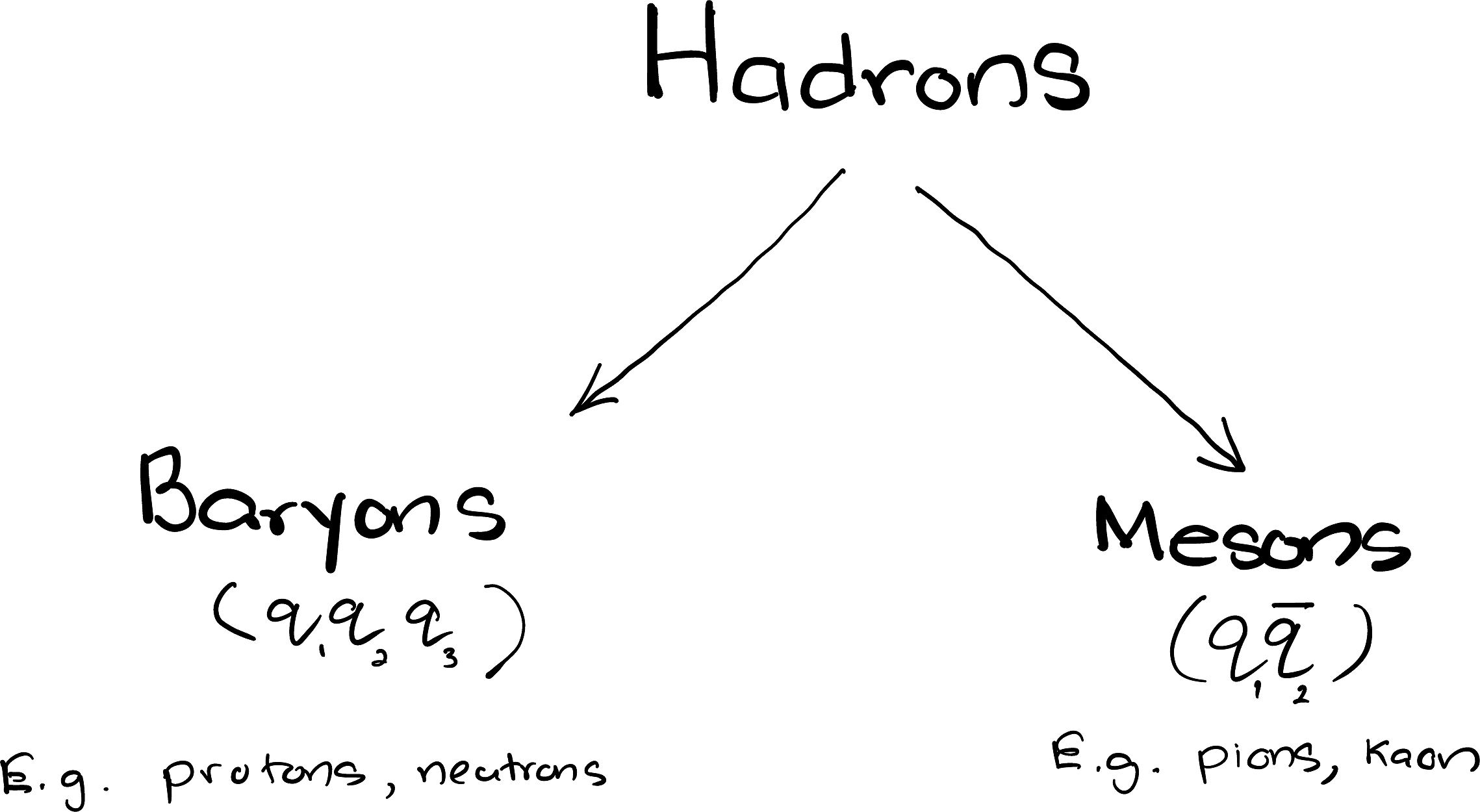
Figure 1.5: Putting quarks together to form baryons and mesons.

Quarks are never observed as free particles. Instead, they are confined within composite particles called hadrons (Figure 1.5). The two most common arrangements are three quarks (\(q_1q_2q_3\)) and a quark–antiquark pair (\(q_1\bar{q}_2\)). We call the three-quark variety baryons (“heavy”) and the quark–antiquark variety mesons (“middle”). The term hadrons (“strong”) collectively refers to both.

The familiar proton and neutron are baryons with the following valence-quark compositions:

\[\begin{align} p &\longrightarrow uud, \\ n &\longrightarrow udd. \end{align}\]

1.5.1 List of Mesons and Baryons

Don’t memorise!

The following tables may seem overwhelming at first glance. Please do not try to memorise all the details. Instead, focus on the patterns in how the quantum numbers are assigned.

Below are lists of some of the baryons (Table 1.8) and mesons (Table 1.9) discovered so far. Please do not try to memorise any of them! I am showing you these tables simply to help you notice the patterns in their quark compositions.

Particle	Spin \(J\)	Quark content	Charge (\(e\))	Mass (\(\mathrm{MeV}/c^2\))	Mean lifetime (s)
\(p\)	\(1/2\)	\(uud\)	\(+1\)	938.272	stable
\(n\)	\(1/2\)	\(udd\)	\(0\)	939.565	\(\sim8.8\times10^{2}\)
\(\Lambda^0\)	\(1/2\)	\(uds\)	\(0\)	1115.683	\(2.63\times10^{-10}\)
\(\Sigma^+\)	\(1/2\)	\(uus\)	\(+1\)	1189.37	\(8.02\times10^{-11}\)
\(\Sigma^0\)	\(1/2\)	\(uds\)	\(0\)	1192.64	\(\sim7.4\times10^{-20}\)
\(\Sigma^-\)	\(1/2\)	\(dds\)	\(-1\)	1197.45	\(1.48\times10^{-10}\)
\(\Xi^0\)	\(1/2\)	\(uss\)	\(0\)	1314.86	\(2.90\times10^{-10}\)
\(\Xi^-\)	\(1/2\)	\(dss\)	\(-1\)	1321.71	\(1.64\times10^{-10}\)
\(\Lambda_c^+\)	\(1/2\)	\(udc\)	\(+1\)	2286.46	\(2.03\times10^{-13}\)
\(\Delta^{++}\)	\(3/2\)	\(uuu\)	\(+2\)	\(\sim1232\)	\(\sim5.6\times10^{-24}\)
\(\Delta^+\)	\(3/2\)	\(uud\)	\(+1\)	\(\sim1232\)	\(\sim5.6\times10^{-24}\)
\(\Delta^0\)	\(3/2\)	\(udd\)	\(0\)	\(\sim1232\)	\(\sim5.6\times10^{-24}\)
\(\Delta^-\)	\(3/2\)	\(ddd\)	\(-1\)	\(\sim1232\)	\(\sim5.6\times10^{-24}\)
\(\Sigma(1385)^+\)	\(3/2\)	\(uus\)	\(+1\)	\(\sim1383\)	\(\sim1.8\times10^{-23}\)
\(\Sigma(1385)^0\)	\(3/2\)	\(uds\)	\(0\)	\(\sim1384\)	\(\sim1.8\times10^{-23}\)
\(\Sigma(1385)^-\)	\(3/2\)	\(dds\)	\(-1\)	\(\sim1387\)	\(\sim1.7\times10^{-23}\)
\(\Xi(1530)^0\)	\(3/2\)	\(uss\)	\(0\)	\(\sim1532\)	\(\sim7.2\times10^{-23}\)
\(\Xi(1530)^-\)	\(3/2\)	\(dss\)	\(-1\)	\(\sim1535\)	\(\sim6.7\times10^{-23}\)
\(\Omega^-\)	\(3/2\)	\(sss\)	\(-1\)	1672.45	\(8.21\times10^{-11}\)

Table 1.8: Table of some baryons

Particle	Spin \(J\)	Quark content	Charge (\(e\))	Mass (\(\mathrm{MeV}/c^2\))	Lifetime (\(\mathrm{s}\))
\(\pi^+\)	\(0\)	\(u\bar{d}\)	\(+1\)	\(139.57\)	\(2.60\times10^{-8}\)
\(\pi^-\)	\(0\)	\(d\bar{u}\)	\(-1\)	\(139.57\)	\(2.60\times10^{-8}\)
\(\pi^0\)	\(0\)	\((u\bar{u}-d\bar{d})/\sqrt{2}\)	\(0\)	\(134.98\)	\(8.43\times10^{-17}\)
\(K^+\)	\(0\)	\(u\bar{s}\)	\(+1\)	\(493.68\)	\(1.24\times10^{-8}\)
\(K^-\)	\(0\)	\(s\bar{u}\)	\(-1\)	\(493.68\)	\(1.24\times10^{-8}\)
\(K_S^0\)	\(0\)	\((d\bar{s}+s\bar{d})/\sqrt{2}\)	\(0\)	\(497.61\)	\(8.95\times10^{-11}\)
\(K_L^0\)	\(0\)	\((d\bar{s}-s\bar{d})/\sqrt{2}\)	\(0\)	\(497.61\)	\(5.12\times10^{-8}\)
\(\eta\)	\(0\)	\(\approx(u\bar{u}+d\bar{d}-2s\bar{s})/\sqrt{6}\)	\(0\)	\(547.86\)	\(5.0\times10^{-19}\)
\(\eta'\)	\(0\)	\(\approx(u\bar{u}+d\bar{d}+s\bar{s})/\sqrt{3}\)	\(0\)	\(957.78\)	\(3.3\times10^{-21}\)
\(D^+\)	\(0\)	\(c\bar{d}\)	\(+1\)	\(1869.66\)	\(1.03\times10^{-12}\)
\(D^-\)	\(0\)	\(d\bar{c}\)	\(-1\)	\(1869.66\)	\(1.03\times10^{-12}\)
\(D^0\)	\(0\)	\(c\bar{u}\)	\(0\)	\(1864.84\)	\(4.10\times10^{-13}\)
\(\bar{D}^0\)	\(0\)	\(u\bar{c}\)	\(0\)	\(1864.84\)	\(4.10\times10^{-13}\)
\(D_s^+\)	\(0\)	\(c\bar{s}\)	\(+1\)	\(1968.35\)	\(5.0\times10^{-13}\)
\(D_s^-\)	\(0\)	\(s\bar{c}\)	\(-1\)	\(1968.35\)	\(5.0\times10^{-13}\)
\(B^+\)	\(0\)	\(u\bar{b}\)	\(+1\)	\(5279.34\)	\(1.64\times10^{-12}\)
\(B^-\)	\(0\)	\(b\bar{u}\)	\(-1\)	\(5279.34\)	\(1.64\times10^{-12}\)
\(B^0\)	\(0\)	\(d\bar{b}\)	\(0\)	\(5279.66\)	\(1.52\times10^{-12}\)
\(\bar{B}^0\)	\(0\)	\(b\bar{d}\)	\(0\)	\(5279.66\)	\(1.52\times10^{-12}\)
\(\rho^+\)	\(1\)	\(u\bar{d}\)	\(+1\)	\(775.1\)	\(\sim4.4\times10^{-24}\)
\(\rho^-\)	\(1\)	\(d\bar{u}\)	\(-1\)	\(775.1\)	\(\sim4.4\times10^{-24}\)
\(\rho^0\)	\(1\)	\((u\bar{u}-d\bar{d})/\sqrt{2}\)	\(0\)	\(775.3\)	\(\sim4.4\times10^{-24}\)
\(K^{*+}\)	\(1\)	\(u\bar{s}\)	\(+1\)	\(891.7\)	\(\sim1.3\times10^{-23}\)
\(K^{*-}\)	\(1\)	\(s\bar{u}\)	\(-1\)	\(891.7\)	\(\sim1.3\times10^{-23}\)
\(K^{*0}\)	\(1\)	\(d\bar{s}\)	\(0\)	\(895.6\)	\(\sim1.4\times10^{-23}\)
\(\bar{K}^{*0}\)	\(1\)	\(s\bar{d}\)	\(0\)	\(895.6\)	\(\sim1.4\times10^{-23}\)
\(\omega\)	\(1\)	\((u\bar{u}+d\bar{d})/\sqrt{2}\)	\(0\)	\(782.7\)	\(\sim7.8\times10^{-23}\)
\(J/\psi\)	\(1\)	\(c\bar{c}\)	\(0\)	\(3096.9\)	\(\sim7.1\times10^{-21}\)
\(D^{*+}\)	\(1\)	\(c\bar{d}\)	\(+1\)	\(2010.3\)	\(\sim7.9\times10^{-21}\)
\(D^{*-}\)	\(1\)	\(d\bar{c}\)	\(-1\)	\(2010.3\)	\(\sim7.9\times10^{-21}\)
\(D^{*0}\)	\(1\)	\(c\bar{u}\)	\(0\)	\(2006.9\)	\(\sim1.2\times10^{-20}\)
\(\bar{D}^{*0}\)	\(1\)	\(u\bar{c}\)	\(0\)	\(2006.9\)	\(\sim1.2\times10^{-20}\)
\(\Upsilon(1S)\)	\(1\)	\(b\bar{b}\)	\(0\)	\(9460.4\)	\(\sim1.2\times10^{-20}\)

Table 1.9: Table of some mesons

1.6 Ingredient 3: Conservation Laws & Colourlessness

In this section, I will focus on the third ingredient of the Standard Model: conservation laws. I will also introduce you to another important property of hadrons called colourlessness.

1.6.1 Conservation Laws

If you stop to think about it, you cannot help but be amazed by the way the Universe conserves certain quantities, such as energy and momentum. These conservation laws are not simply a collection of useful bookkeeping rules. Many of them arise from the fundamental symmetries of our Universe.

The connection between symmetries and conservation laws has a firm mathematical foundation and is captured by Noether’s theorem. This fascinating topic is beyond the remit of this course. However, Dr Alex Hue has kindly written some supplementary notes on Noether’s theorem for those of you who would like to explore it further.

Here is a list of some of the conservation laws that we will deal with in this course.

Some conserved quantities
Always Conserved	Conserved When No Weak Interaction
Energy	Downness (\(D\))
Linear and angular momentum	Upness (\(U\))
Electric charge (\(Q\))	Strangeness (\(S\))
Electron number (\(L_e\))	Charmness (\(C\))
Muon number (\(L_\mu\))	Bottomness (\(B\))
Tau number (\(L_\tau\))	Topness (\(T\))
Baryon number (\(A\))

As we shall see, not every quantity is conserved in every type of interaction. Whenever we examine a particle reaction, we must therefore ask two questions: 1. what type of interaction is responsible, and 2. what quantities might be conserved.

1.6.2 Colourlessness

Let’s now talk about a fascinating property of hadrons. Recall that quarks carry colour charge. There are three possible colours, which we rather imaginatively call red (\(R\)), green (\(G\)), and blue (\(B\)).

A baryon contains three quarks (for example, a proton has the quark content \(uud\)). We can picture one possible colour assignment for the proton as a red up quark (\(\rq{u}\)), a green up quark (\(\gq{u}\)), and a blue down quark (\(\bq{d}\)):

\[ p\longrightarrow\rq{u}\gq{u}\bq{d}. \tag{1.4}\]

The resulting proton is described as colourless because the three colours combine to form a colour-neutral state. The familiar idea that \(R+G+B\) produces white light gives us a useful way to remember this.

Do not take the analogy too literally, though. Colour charge has nothing to do with the colours that we see, and the quarks do not permanently carry the particular colours shown above. The proton is actually a quantum superposition of the possible colour assignments. What matters is that the complete combination is colourless.

And now comes the remarkable part: Mother Nature insists that all directly observable particles be colourless.

All directly observable particles are colourless

Using colours to represent the strong charge gives us a delightfully simple way to picture how hadron exist. For instance, for a meson to be colourless, a quark of one colour must be paired with an antiquark carrying the corresponding anticolour.

Consider, the specific example of a \(\pi^+\) meson, which has the flavour content \(u\bar{d}\). One possible colour combination consists of a red up quark and an antired anti-down quark:

\[ \pi^+\longrightarrow\rq{u}\,\overline{\rq{d}}. \tag{1.5}\]

The red and antired colour charges cancel, leaving a colourless pion. However, just as with the proton, this is not the whole story. The colour part of the pion’s state is actually a superposition of all three possible colour–anticolour combinations. So, a better representation is:

\[ \pi^+\longrightarrow \frac{\rq{u}\,\overline{\rq{d}} + \gq{u}\,\overline{\gq{d}} + \bq{u}\,\overline{\bq{d}}}{\sqrt{3}}. \]

When we are interested only in its quark flavours, we simply write

\[ \pi^+ = u\bar{d}. \tag{1.6}\]

1.7 How Many Gluons?

Let’s quickly talk about gluons, the mediators of the strong interaction.

Unlike photons which carry no charge, gluons themselves carry the colour charge associated with the interaction they mediate. More specifically, a gluon carries a combination of colour and anticolour, which we can write schematically as \(C\bar{C}\). With three colours, we might therefore expect \(3\times3=9\) possible combinations: \[ \begin{matrix} r\bar{r} & r\bar{g} & r\bar{b} \\ g\bar{r} & g\bar{g} & g\bar{b} \\ b\bar{r} & b\bar{g} & b\bar{b} \end{matrix} \tag{1.7}\]

However, these colours represent quantum states, and a gluon does not generally exist in just one of the individual colour–anticolour states listed above. Instead, the physical gluon states can be represented by orthogonal linear combinations of them.

\[ \newcommand\fx[4]{\f{#1\b{#2} - #3\b{#4}}{\sqrt{2}}} \] \[ \begin{matrix} \fx{r}{b}{b}{r} && -\fx{r}{b}{b}{r} \\ \fx{r}{g}{g}{r} && -\fx{r}{g}{g}{r} \\ \fx{r}{g}{g}{b} && -\fx{r}{g}{g}{b} \\ \fx{r}{r}{b}{b} && -\f{r\b{r}+b\b{b} - 2g\b{g}}{\sqrt{6}} \\ % &\cancelto{\text{ colourless}}{\f{1}{\sqrt{2}}\lr{r\b{r}+b\b{b} +g\b{g}}}& \end{matrix} \tag{1.8}\]

That gives us eight independent gluon states. But what happened to the ninth combination? The remaining orthogonal combination is

\[ \frac{r\bar{r}+g\bar{g}+b\bar{b}}{\sqrt{3}}. \tag{1.9}\]

This is called a colour-singlet state. It is a bit analogous to a spin-singlet state².

The strong interaction requires colour states to change in a particular way, governed by the symmetry group \(SU(3)\)³ The singlet remains unchanged under these colour transformations and therefore does not correspond to one of the possible gluon states. So, we have a total of eight gluons!

If you like more details, Alex has also prepared a note on the gluon states.

1.8 A Quick Word About Quantum Fields

Before moving on, let me give you an intuitive picture of a quantum field, without the mathematics.

In non-relativistic quantum mechanics, we usually begin with a fixed number of particles and ask questions such as, “Where is the particle likely to be?” This works very well at low energies. At sufficiently high energies, however, particles can be created and destroyed. The number of particles is no longer fixed, so our description must be able to accommodate particles appearing and disappearing. This is one reason why we need quantum field theory (QFT).

The Standard Model associates a quantum field with every type of elementary particle. There is an electron field, a photon field (the electromagnetic field), a quark field for each flavour, and so on. These fields fill all of space, even where no particles are present. What we experience as a particle is a discrete excitation, or quantum, of the corresponding field. A photon is an excitation of the electromagnetic field, while an electron is an excitation of the electron field. Roughly speaking, exciting a field once gives us one particle, exciting it twice gives us two particles, and so on.

QFT has creation operators to add particles to a field and annihilation operators to remove them. This is how QFT allows particles to appear or disappear during an interaction. Instead of following a fixed collection of particles throughout an interaction, QFT instead asks for the probability of one initial state transforming into a particular final state. For example,

\[ e^+e^- \longrightarrow \gamma\gamma \tag{1.10}\]

describes an electron and a positron annihilating to produce two photons. QFT allows us to calculate the probability that this process will occur. Feynman diagrams are one way to calculate these probabilities.

There is another important part of the story: quantum fields can interact, or couple, with one another. For example, the electron field couples to the electromagnetic field. This coupling allows electrons to emit and absorb photons and, therefore, allows photons to mediate the electromagnetic interaction between charged particles.

However, not every field couples directly to every other field. The pattern and strength of these couplings determine which particles can interact and how strongly they do so.

The Higgs field is an especially important example. The electron field couples to the Higgs field, and this interaction gives the electron its mass. The stronger an elementary particle couples to the Higgs field, the greater the mass it acquires. Photons and gluons do not couple to the Higgs field, so they are massless.

1.9 A Final Tally

Let’s round up by making a final tally. To do this, we should not forget the most famous one: the Higgs boson.

The Higgs boson (\(H\)) has a mass of about \(M_H=125~\mathrm{GeV}/c^2\) and a spin of 0. It stands out as the only elementary spin-0 particle discovered so far. There are other spin-0 particles, such as pions, but these are composite particles.

I began by claiming that there were “about” 12 fundamental fermions running the show. Clearly, that was only the beginning of the story. Once we count the antiparticles, colour states, force carriers and the Higgs boson, our accounting gives us a grand total of 61 elementary particle states!

The final particle count of the Standard Model
Quarks (in three colours)	\(6\times3 = 18\)
Leptons	\(6\)
AntiQuarks (in three colours)	\(6\times3 = 18\)
AntiLeptons	\(6\)
Gluons	\(8\)
Gauge bosons	\(4\)
Higgs	\(1\)
	\(61\)

Do not become too attached to the number 61, though. The final total depends on exactly what we choose to count separately (for example, whether we count antiparticles, colour states, and gluon states individually). The important point is not the number itself, but how a small number of particles, together with the interactions and symmetries of the Standard Model, gives rise to the wonderfully rich Universe we live in.

That is enough for now. In the next lecture, I will discuss how we figured out the various features described so far and, more importantly, see them in action.

References

Jaeger, G. Are Virtual Particles Less Real? Entropy 21, 141 (2019).

Chapter Footnotes

Called Møller scattering↩︎
\(\frac{\uparrow\downarrow-\downarrow\uparrow}{\sqrt{2}}\)↩︎
We will not explore \(SU(3)\) in this course.↩︎