Worked Examples 2
\[ \newcommand\v[1]{\boldsymbol{#1}} \newcommand\vdot[2]{\v{#1}\cdot\v{#2}} \]
\[ \newcommand{\dd}[2][]{\mathrm{d}^{#1}#2} \]
\[ \newcommand\f[2]{\dfrac{#1}{#2}} \newcommand\da[2]{\dfrac{d #1}{d #2}} \newcommand\daa[2]{\dfrac{d^2 #1}{d #2^2}} \newcommand\pa[2]{\dfrac{\partial #1}{\partial #2}} \newcommand\pal[3]{\left.\dfrac{\partial #1}{\partial #2}\right|_{#3}} \newcommand\paa[2]{\dfrac{\partial^2 #1}{\partial #2^2}} \newcommand\pab[3]{\dfrac{\partial^2 #1}{\partial #2 \partial #3}} \def\half{\frac{1}{2}} \]
\[ \newcommand\ket[1]{\left|#1\right\rangle} % |x> \newcommand\exp[1]{\left\langle#1\right\rangle} % <x> \newcommand\lr[1]{\left(#1\right)} % (x) \newcommand\lrs[1]{\left[#1\right]} % [x] \newcommand\lra[1]{\left|#1\right|} % |x| \newcommand\lrc[1]{\left\{#1\right\}} % {x} \newcommand\lrl[3]{\left.#1\right|_{#2}^{#3}} % x_limits \]
\[ \def\ie{\text{i.e.}\quad} \]
\[ \newcommand{\me}[3][\rightarrow]{{#2}#1{#3}} % Typical reaction \newcommand{\nr}[3]{{#1}\,({#2})\,{#3}} % Nuclear reactions \newcommand{\ele}[4]{_{#2}^{#3}{\textbf{#1}}_{#4}} \newcommand{\el}[2]{^{#2}\text{#1}} \newcommand{\til}[2][\mathbf{\sim}]{\underset{#1}{{#2}}} \newcommand{\b}[1]{\overline{#1}} \]
\[ \newcommand{\coulomb}[1]{\dfrac{#1}{4\pi\epsilon_0}} \def\degree{^*} \]
\[ \def\amu{\text{ amu}} \def\J{\text{ J}} \def\K{\text{ K}} \def\s{\text{ s}} \def\second{\text{ s}} \def\Psecond{\text{ s}^{-1}} \def\m{\text{ m}} \def\mm{\text{ mm}} \def\km{\text{ km}} \def\fm{\text{ fm}} \def\mum{\text{ $\mu$m}} \def\mus{\text{ $\mu$s}} \def\mPERs{\text{ ms$^{-1}$}} \def\eV{\text{ eV}} \def\keV{\text{ keV}} \def\GeV{\text{ GeV}} \def\MeV{\text{ MeV}} \def\MeVc{\text{ MeV/c$^2$}} \def\KeVc{\text{ KeV/c$^2$}} \newcommand\ttp[1]{\times 10^{#1}} % To The Power \]
\[ \def\en{\nu_e} \def\Aen{\b{\nu_e}} \def\mun{\nu_\mu} \def\Amun{\b{\nu}_\mu} \]
\[ \def\uraniumA{\ele{U}{92}{233}{}} \def\uraniumB{\ele{U}{92}{235}{}} \def\uraniumC{\ele{U}{92}{238}{}} \def\carbonB{\ele{C}{6}{14}{}} \def\nitrogenB{\ele{N}{7}{14}{}} \def\oxygenA{\ele{O}{8}{14}{}} \def\oxygenB{\ele{O}{8}{16}{}} \]
\[ % \def\com{\text{\scriptsize CM}} \def\com{\mathrm{\scriptsize CM}} \]
\[ \def\l{l} \]
\[ \def\g{\gamma} \]
Example 1 (Meson decay)
A \(\pi^0\) meson is moving in laboratory frame with kinetic energy \(r\,mc^2\), decays into two photons of equal energy. Where \(m\) is the rest mass of the meson and \(r\) is a positive constant.
Determine the opening angle \(\theta\) between the photon directions.
Solution 1 (Meson decay).
- \(E_0\) and \(\vec{p}_0\) be the total energy and momentum of the meson.
- \(E\) and \(\vec{p}\) be the energy and momentum of one of the photons.
Since, \[ E^2 = p^2c^2 + m^2c^4, \]
we have
\[ E_0^2 = p_0^2c^2 + m^2c^4 \tag{1}\]
with
\[ E_0 = (1+r)mc^2 \tag{2}\]
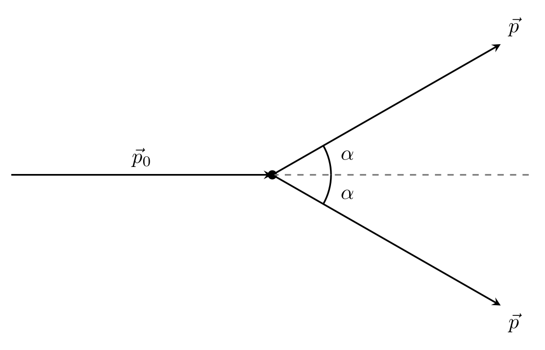
Let:
and, for a photon,
\[ E = pc. \tag{3}\]
Energy and momentum are conserved:
\[ 2E = E_0 \]
and
\[ 2p\cos\alpha = p_0. \]
Therefore,
\[ \cos\alpha = \frac{p_0}{2p} = \frac{p_0}{2E/c} = \frac{p_0c}{E_0}. \]
Hence,
\[ \cos^2\alpha = \frac{p_0^2c^2}{E_0^2} = 1-\frac{m^2c^4}{E_0^2}= 1-\frac{1}{(1+r)^2}. \]
\[ \Rightarrow\sin\alpha=\frac{1}{1+r}. \]
Therefore, the opening angle is
\[ \theta = 2\sin^{-1}\left(\frac{1}{1+r}\right) \]
Example 2 (JJ Coupling vs LS Coupling of Angular Momentum)
Consider a system of \(N\) distinguishable particles, each possessing orbital angular momentum \(\mathbf{l}_i\) and spin angular momentum \(\mathbf{s}_i\). The total angular momentum may be constructed using either the \(jj\)-coupling scheme or the \(LS\)-coupling scheme.
| Coupling scheme | Construction |
|---|---|
| \(jj\) coupling | \(\mathbf{J}=\sum_{i=1}^{N}\mathbf{j}_i\), where \(\mathbf{j}_i=\mathbf{l}_i+\mathbf{s}_i\) |
| \(LS\) coupling | \(\mathbf{J}=\mathbf{L}+\mathbf{S}\), where \(\mathbf{L}=\sum_{i=1}^{N}\mathbf{l}_i\) and \(\mathbf{S}=\sum_{i=1}^{N}\mathbf{s}_i\) |
Now consider a system containing two distinguishable particles with the following angular-momentum quantum numbers:
| Particle | \(l_i\) | \(s_i\) |
|---|---|---|
| 1 | \(1\) | \(1\) |
| 2 | \(4\) | \(\f12\) |
Using the \(jj\)-coupling scheme, determine the multiplicity with which each possible value of the total angular-momentum quantum number \(J\) occurs.
Show the allowed intermediate values of \(j_1\) and \(j_2\).Repeat the calculation using the \(LS\)-coupling scheme.
Show the allowed intermediate values of \(L\) and \(S\).Verify that the two coupling schemes give the same multiplicity for each possible value of \(J\).
In no more than 50 words, explain why the two coupling schemes must give the same result.
Please show your working.
Solution 1.3.
\[ \def\three{\textcolor{Orange}{\f32}} \def\five{\textcolor{BrickRed}{\f52}} \def\seven{\textcolor{Purple}{\f72}} \def\nine{\textcolor{RoyalBlue}{\f92}} \def\eleven{\textcolor{TealBlue}{\f{11}2}} \def\thirteen{\textcolor{ForestGreen}{\f{13}2}} \]
JJ Coupling vs LS Coupling of Angular Momentum
\(jj\) coupling
Determining \(j_i\)
| Particle | \(l_i\) | \(s_i\) | Range | \(j_i\) |
|---|---|---|---|---|
| 1 | \(1\) | \(1\) | \(0\to2\) | \(0,1,2\) |
| 2 | \(4\) | \(\f12\) | \(\f72\to \f92\) | \(\f72,\f92\) |
Determining \(j\)
| \(j_1\) | \(j_2\) | Range | \(j\) |
|---|---|---|---|
| 0 | \(\f72\) | \(\f72\) | \(\seven\) |
| 1 | \(\f72\) | \(\f52\to\f92\) | \(\five,\seven,\nine\) |
| 2 | \(\f72\) | \(\f32\to\f{11}2\) | \(\three,\five,\seven,\nine,\eleven\) |
| 0 | \(\f92\) | \(\f92\) | \(\nine\) |
| 1 | \(\f92\) | \(\f72\to\f{11}2\) | \(\seven,\nine,\eleven\) |
| 2 | \(\f92\) | \(\f52\to\f{13}2\) | \(\five,\seven,\nine,\eleven,\thirteen\) |
Multiplicities
| \(j\) | \(\three\) | \(\five\) | \(\seven\) | \(\nine\) | \(\eleven\) | \(\thirteen\) |
|---|---|---|---|---|---|---|
| # | \(1\) | \(3\) | \(5\) | \(5\) | \(3\) | \(1\) |
\(LS\) coupling
Determining \(l\)
| \(l_1\) | \(l_2\) | Range | \(l\) | |
|---|---|---|---|---|
| \(l\) | \(1\) | \(4\) | \(3\to5\) | \(3,4,5\) |
Determining \(s\)
| \(s_1\) | \(s_2\) | Range | \(s\) | |
|---|---|---|---|---|
| \(s\) | \(1\) | \(\f12\) | \(\f12\to\f32\) | \(\f12,\f32\) |
Determining \(j\)
| \(l\) | \(s\) | Range | \(j\) |
|---|---|---|---|
| 3 | \(\f12\) | \(\f52\to\f72\) | \(\five,\seven\) |
| 4 | \(\f12\) | \(\f72\to\f92\) | \(\seven,\nine\) |
| 5 | \(\f12\) | \(\f92\to\f{11}2\) | \(\nine,\eleven\) |
| 3 | \(\f32\) | \(\f32\to\f92\) | \(\three,\five,\seven,\nine\) |
| 4 | \(\f32\) | \(\f52\to\f{11}2\) | \(\five,\seven,\nine,\eleven\) |
| 5 | \(\f32\) | \(\f72\to\f{13}2\) | \(\seven,\nine,\eleven,\thirteen\) |
Multiplicities
| \(j\) | \(\three\) | \(\five\) | \(\seven\) | \(\nine\) | \(\eleven\) | \(\thirteen\) |
|---|---|---|---|---|---|---|
| # | \(1\) | \(3\) | \(5\) | \(5\) | \(3\) | \(1\) |
Here are two valid reasons:
- The total-angular-momentum states form a Hilbert space. The \(jj\)- and \(LS\)-coupling schemes are two different bases for this same space. Therefore, they must contain the same number of states with each value of \(J\).
- How we choose to couple the constituent angular momenta cannot change the number of physical states obtained.
Example 1.1 (Alpha-decay selection rules)
Nuclei, like atoms, possess discrete energy levels. The spin and parity of a nucleus depend on the energy state occupied by the nucleus. These states are conventionally labelled using the notation \(J^\eta\).
Consider a parent nucleus that decays directly into a daughter nucleus by emitting an \(\alpha\)-particle. Alpha decay conserves total angular momentum and parity.
The parent nucleus is initially in a \(0^+\) state. An \(\alpha\)-particle has spin-parity \(0^+\) and may carry orbital angular momentum \(\ell_\alpha\) relative to the daughter nucleus.
The figure shows four energetically accessible daughter states.
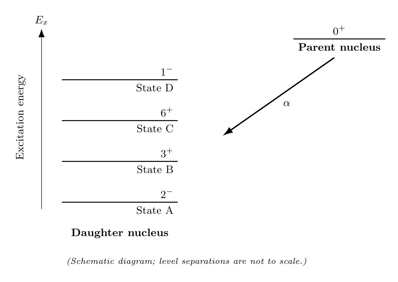
For each daughter state shown:
- Determine the required value of \(\ell_\alpha\).
- Decide whether the transition is allowed or forbidden.
- Hence, state the general pattern of daughter-state spin-parities that can be reached through \(\alpha\)-decay from a \(0^+\) parent nucleus.
Please explain your reasoning.
Solution 1.2 (Alpha-decay selection rules).
Consider the conservation of angular momentum:
The total angular momentum of the parent nucleus is zero. Therefore, the total angular momentum after the decay must also be zero.
After the decay, the total angular momentum is obtained by coupling the spin \(\vec{J}_D\) of the daughter nucleus with the relative orbital angular momentum \(\vec{\ell}_\alpha\) of the daughter–\(\alpha\) system.
Since the \(\alpha\)-particle has spin zero, it makes no intrinsic-spin contribution.
For \(\vec{J}_D\) and \(\vec{\ell}_\alpha\) to couple to zero, their angular-momentum quantum numbers must be equal:
\[ \ell_\alpha=J_D. \]
Since parity is also conserved, the total parity of the system after the decay is
\[ \begin{aligned} \eta_{\text{after}} &= (-1)^{\ell_\alpha} \eta_{\text{daughter}} \eta_\alpha \\ &= (-1)^{\ell_\alpha} \eta_{\text{daughter}}(+1) \\ &= (-1)^{J_D} \eta_{\text{daughter}}. \end{aligned} \]
The parent nucleus has positive parity. Therefore, parity conservation requires
\[ \eta_{\text{after}}=+1. \]
This condition is satisfied only by daughter states with
- odd \(J_D\) and negative parity; or
- even \(J_D\) and positive parity.
Hence, the daughter states accessible through \(\alpha\)-decay from a \(0^+\) parent follow the pattern
\[ J_D^{\eta_D} = 0^+,\ 1^-,\ 2^+,\ 3^-,\ 4^+,\ldots \]
Therefore:
| State | \(J_D^{\eta_D}\) | \(\ell_\alpha\) | Total parity after decay \((-1)^{J_D} \eta_{\text{daughter}}\) |
Result |
|---|---|---|---|---|
| A | \(2^-\) | \(2\) | \(-\) | Forbidden |
| B | \(3^+\) | \(3\) | \(-\) | Forbidden |
| C | \(6^+\) | \(6\) | \(+\) | Allowed |
| D | \(1^-\) | \(1\) | \(+\) | Allowed |
Example 1.2 (\(\gamma\) Spectrum from \(\beta^+\) Sample)
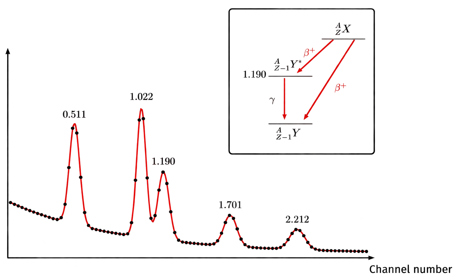
The figure shows the \(\gamma\)-ray spectrum measured by a detector observing the \(\beta^+\) (\(e^+\)) decay of \({}^{A}_{Z}\mathrm{X}\) to \({}^{A}_{Z-1}\mathrm{Y}\) (shown in the inset).
The first excited state of \({}^{A}_{Z-1}\mathrm{Y}^{*}\) lies at an energy of 1.190 MeV, so only a single nuclear \(\gamma\) transition is expected. However, multiple peaks are observed in the measured spectrum.
Identify possible physical origins of each of the five labelled peaks in the spectrum. Please explain your reasoning.
Notes
- The figure is schematic and shows only the five peaks relevant to this question.
- The labels indicate the energy deposited in the detector.
- All energies are given in MeV.
- The detector is assumed to record photons only. Energy deposited by charged particles is not recorded.
- Pair production by the \(\gamma\) ray in the detector, the associated escape peaks, and Compton effects may be neglected.
- Assume that the detector surrounds the sample and records the total energy deposited by photons arriving within its resolving time as a single event.
Solution 1.3.
Let \(E_\gamma\) denote the energy of the nuclear photon. The peak at \(E_\gamma\) arises from full absorption of the photon emitted when the excited daughter nucleus relaxes to its ground state.
The positron emitted in the \(\beta^+\) decay slows down and annihilates with an electron. For two-photon annihilation approximately at rest, each photon has energy \[ E_{\mathrm{annihilation}} = m_e c^2 = 0.511\,\mathrm{MeV}. \]
One or both of these photons may leave the sample and be absorbed in the surrounding detector.
The detector records the total energy deposited within its resolving time as a single event. Thus, full absorption of different combinations of the nuclear photon and the two annihilation photons gives the five labelled peaks:
| Photons fully absorbed in one event | Recorded energy (MeV) |
|---|---|
| One annihilation photon only | \(0.511\) |
| Both annihilation photons only | \(1.022\) |
| Nuclear photon only | \(E_\gamma\) |
| Nuclear photon and one annihilation photon | \(E_\gamma + 0.511\) |
| Nuclear photon and both annihilation photons | \(E_\gamma + 1.022\) |
For example, for \(E_\gamma=1.190\,\mathrm{MeV}\), the last two peaks occur at \(1.701\,\mathrm{MeV}\) and \(2.212\,\mathrm{MeV}\).