3 Importance of Angular Momentum*

What To Expect In This Chapter

The quantum mechanics of angular momentum plays an essential in the description of nuclear and particle physics. So we need to review the quantum mechanical theory of angular momentum, especially how the angular momenta of several particles can be added. This is necessary to understand many of the other topics we will discuss in this course. So, in this chapter, I will take you on another whirlwind tour, this time of angular momentum. I will also touch on the quantum mechanical ideas of identical particles because elementary particles are identical.

I am only motivated by the need to use these ideas in our course, so the quantum mechanical forays will not be in any sense complete. However, if you are keen on a more in-depth discussion, don’t worry Dr Alex($\uparrow$) Hue has thoughtfully prepared some detailed(optional **) reference notes for you. They can be found in chapter Quantum Mechanics Reference in the Supplementary Material.

3.1 Central Potentials: A Simple Place to Start

A typical approach to solving the Schrödinger equation in three dimensions is to consider a central potential and separate the wave function into radial $R(r)$ and angular $\Theta(\theta)\Phi(\phi)$ portions¹ .

\[ \psi(r,\theta,\phi) \equiv R(r)\Theta(\theta)\Phi(\phi) \]

The angular solutions are the spherical harmonics $Y^{m}_\l(\theta,\phi)$:

\[ \Theta(\theta)\Phi(\phi) \equiv Y^{m}_\l(\theta,\phi) \]

The explicit form of the spherical harmonics is:

\[ Y^{m}_\l(\theta,\phi) = \xx\times \sqrt{\frac{2\l+1}{4\pi}\frac{(\l-\lra{m})!}{(\l+\lra{m})!}} e^{im\phi}P_{\l}^{m}(\cos\theta) \tag{3.1}\]

where $P^m_\l(x)$ are the Associated Legendre functions given by \[ P^m_\l(x) = (1-x^2)^{|m|/2}\lr{\da{}{x}}^{|m|}P_\l(x) \tag{3.2}\]

and $P_\l(x)$ is the $\l$th Legendre polynomial

\[ P_\l(x) = \frac{1}{2^l l!} \frac{d^l}{dx^l} (x^2-1)^l \]

3.1.1 Quantisation

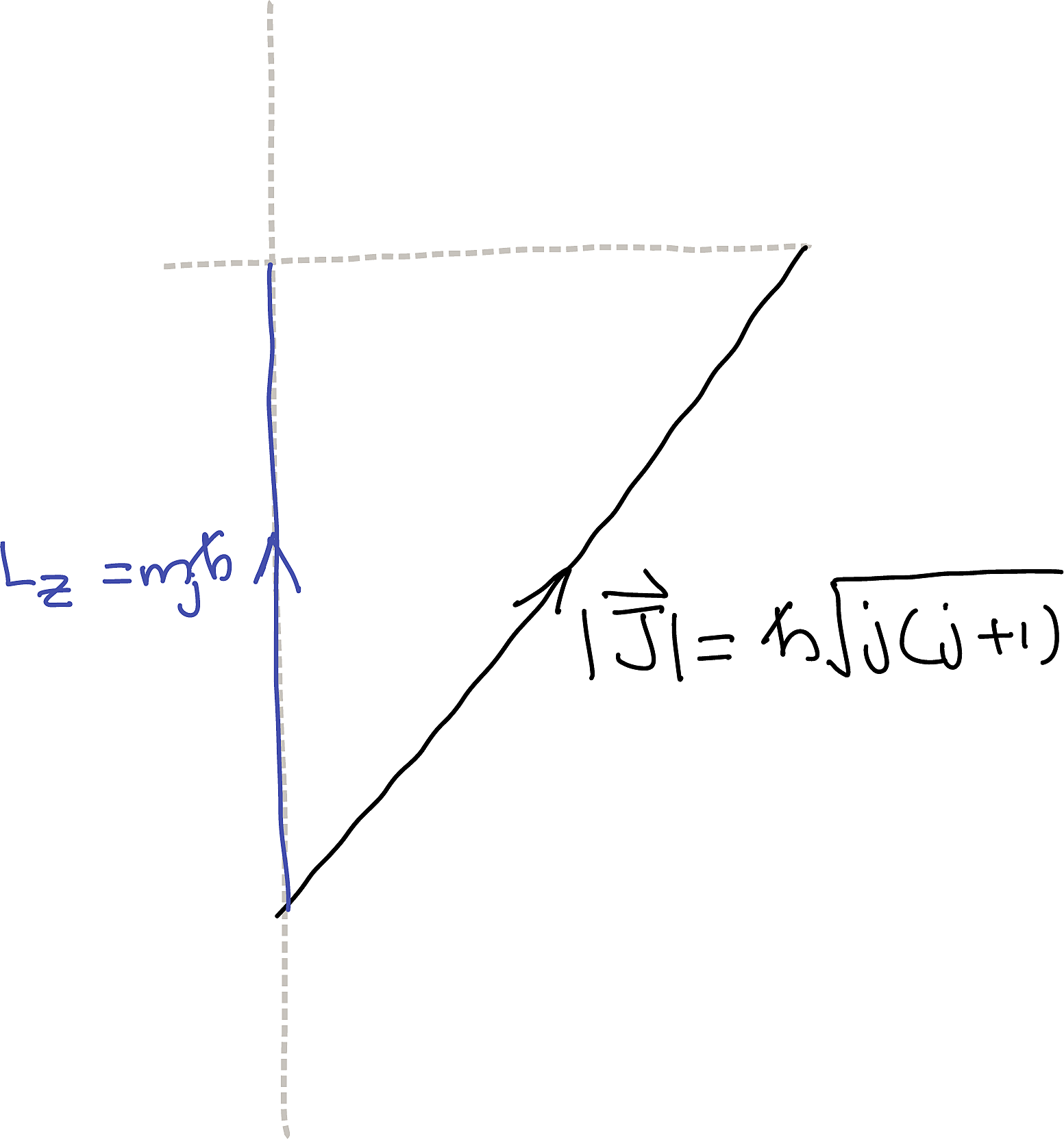
There are restrictions on the values that $\l$ and $m$ can take. The restrictions on $m$ arise from insisting that $\Phi(\phi)=\Phi(2m\pi+\phi)$ which introduces the quantisation of $m$. Later, this leads to the restriction on $\l$, forcing it to assume only non-negative integer values. Ultimately, we are left with the result that angular momentum is quantised such that:

\[ \begin{array}{ccll} |\v{L}| &=& \hbar\sqrt{\l(\l+1)}&\qquad&(\l=0,1,2,\ldots) \\ L_z &=& m\hbar&\qquad&(m=-\l,-\l+1,\ldots,\l-1,+\l) \end{array} \tag{3.3}\]

So, for a given $\l$, there are $(2\l+1)$ possible values of $L_z$ where $m$ runs from $-\l$ to $+\l$ in integer steps. It is also common to use spectroscopic notation to refer to the various angular momentum states.

$\l$	0	1	2	3	4	5
Notation	$s$	$p$	$d$	$f$	$g$	$h$

3.1.2 Physical Interpretation

It is good to understand what this result means for measurements. Let’s consider a simple system like the hydrogen atom in an excited state (because the ground state is a tad boring). If you measure the total angular momentum ($|\v{L}|$) of such a system, you will always get the value $\hbar\sqrt{\l(\l+1)}$. Following this measurement, if you measure only the $z$-component of the angular momentum (i.e. $L_z$), you will get a value $m\hbar$. Now, the nice thing is, that if you go back and measure $|\v{L}|$, you will get the same value as before. This happens because the corresponding operators commute:

\[ [\hat{L}, \hat{L_z}]=0 \]

I.e. we can have simultaneous measurements of both these quantities. So, you can consider both these values as resulting from a single measurement of the two properties.

3.2 A More General Analysis Of Angular Momentum

Since the quantisation of $m$ is based on physical grounds, it turns out that the above analysis misses out on some solutions. A more general analysis of angular momentum based on just the operators and commutator relations (see [Alex’s notes]{extra_qm_alex.qmd}) leads to the more general version of Equation 3.3, which is:

\[ \begin{array}{ccll} |\v{J}| &=& \hbar\sqrt{j(j+1)}&\qquad&(j=0,\frac{1}{2},1,\frac{3}{2},2,\frac{5}{2},\ldots) \\ J_z &=& m_j\hbar&\qquad&(m_j=-j,-j+1,\ldots,j-1,+j) \end{array} \tag{3.4}\]

Kindly note:

I switched to using the symbols $\v{J}$ and $j$ to refer to this more general result of angular momentum.
For a given $j$, there are $(2j+1)$ possible values of $J_z$ where $m_j$ runs from $-j$ to $+j$ in integral steps.
Half-integer values are now allowed for the quantum number $j$.
These correspond to spin angular momentum states that don’t appear in the previous analysis, as spin has no physical counterpart.

3.3 Angular Momentum Addition Theorem

When a system has multiple forms of angular momenta (e.g., orbital, spin) or when there are multiple particles, the total angular moment is more important as it is the quantity that is conserved. So, we need to understand the quantum mechanical recipe for adding different angular momenta. This is called the Angular Momentum Addition Theorem. Let me demonstrate this by considering two angular momenta $\v{J_1}$ and $\v{J_2}$ of two particles.

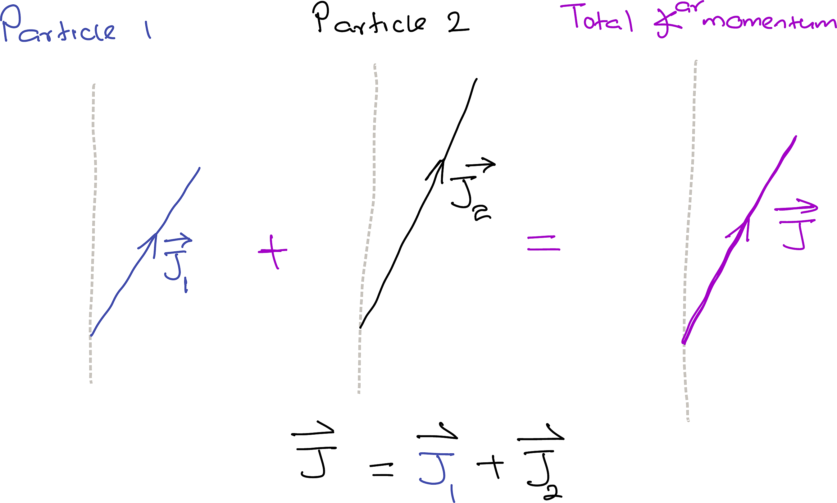
The total angular momentum is $\v{J} = \v{J_1} + \v{J_2}$ and being an angular momentum, is itself quantised. How $\v{J}$ is quantised depends on the states of both $\v{J_1}$ and $\v{J_2}$. How all this works out is shown below.

\[\begin{array}{l|l|l} \text{Angular momentum 1 ($\v{J_1}$)}&\text{Angular momentum 2 ($\v{J_2}$)}&\text{Total Angular momentum ($\v{J}$)}\\ \hline |\v{J_1}|=\hbar\sqrt{j_1(j_1+1)}&|\v{J_2}|=\hbar\sqrt{j_2(j_2+1)}&|\v{J_1}|=\hbar\sqrt{j(j+1)}\\ j_1 = 0, 1, 2,\ldots&j_2 = 0, 1, 2,\ldots& j = |j_2-j_1|, \ldots,(j_1+j_2)\\ && \ie |j_2-j_1|\leq j\leq (j_1 + j_2)\\[1.125em] J_{1z}=m_1\hbar&J_{2z}=m_2\hbar&J_{z}=m_j\hbar\\ \underbrace{m_1=-j_1,\ldots,+j_1}_{\text{$2j_1+1$ values}}&\underbrace{m_2=-j_2,\ldots,+j_2}_{\text{$2j_2+1$ values}}&\underbrace{m=-j,\ldots,+j}_{\text{$2j+1$ values}} \end{array}\]

3.3.1 The tale of two electrons

Let’s now look at a more specific example of a two-electron system. To simplify matters, let’s contused take them to be in the $\l=0$ (i.e. $s$) spatial angular momentum so that we can focus on only spin angular momentum.

\[\begin{array}{cccc} &\text{Electron 1} & \text{Electron 2}& \text{System} \\ \hline &&& |s_1-s_2| \leq s \leq (s_1+s_2) \\ \text{Spin quantum number}& s_1 = \frac{1}{2}& s_2 = \frac{1}{2}& |\frac{1}{2}-\frac{1}{2}| \leq s \leq (\frac{1}{2}+\frac{1}{2}) \\ & & & s=0,1\\ \hline \text{Size of angular momentum} & |\v{S_1}| = \hbar\sqrt{s_1(s_1+1)} & |\v{S_2}| = \hbar\sqrt{s_2(s_2+1)} & |\v{S}| = 0 \text{ or } \sqrt{2}\hbar\\[3em] \hline \text{$z$ component ($\hbar m_x$)}& m_{1z} =-\frac{1}{2},+\frac{1}{2} & m_{2z} =-\frac{1}{2},+\frac{1}{2}& m = \begin{cases}0 & (\text{Singlet})\\-1,0,1 & (\text{Triplet})\end{cases}\\ \hline \end{array}\]

3.4 Labelling Angular Momentum States & CSCO

We can represent the previous two-electron system as uncoupled states

\[ % \newcommand\s[2]{\left|\color{darkorange}{\tp},{#1},\color{red}{\tp}\,{#2}\right\rangle} \newcommand\s[2]{\ket{\spin,#1,\spin,#2}} \newcommand\ss[2]{\ket{#1,#2}} \t{\colourme{s_1},m_1,\colourme{s_2},m_2}= \begin{cases} \s{\tp}{\tp}\longrightarrow\ss{\ttp}{\ttp}\\ \s{\tp}{\tn}\longrightarrow\ss{\ttp}{\ttn}\\ \s{\tn}{\tp}\longrightarrow\ss{\ttn}{\ttp}\\ \s{\tn}{\tn}\longrightarrow\ss{\ttn}{\ttn}\\ \end{cases} \]

or coupled states:

\[ % \newcommand\s[2]{\left|{#1},{#2},\color{darkorange}{\tp},\color{darkorange}{\tp}\right\rangle} \newcommand\s[2]{\ket{#1,#2,\spin,\spin}} \newcommand\ss[2]{\ket{#1,#2}} \t{s,m,\colourme{s_1},\colourme{s_2}}= \begin{cases} \s{0}{\;\;\,0}\longrightarrow\ss{0}{\;\;\,0}\\ \s{1}{-1}\longrightarrow\ss{1}{-1}\\ \s{1}{\;\;\,0}\longrightarrow\ss{1}{\;\;\,0}\\ \s{1}{\;\;\,1}\longrightarrow\ss{1}{\;\;\,1}\\ \end{cases} \]

Note that the number of states (4) is the same in both coupled and uncoupled representations and you can use either representation. These are examples of a complete set of commuting observables (CSCO). They are complete because they allow us to uniquely identify the state of the system. The idea here is to use as many compatible observables to uniquely identify the various states of a system.

3.4.1 Explicit form for the states

Let’s now look at the explicit form of the coupled states in terms of the uncoupled states. You can move from one representation to the other via two routes. The first is by using the Clebsch-Gordan coefficients ($c^j_{m_1,m_2}$) shown in Equation 3.5 below. The second is by using ladder operators.

\[ \t{j,m_j,j_1,j_2} = \sum_{m_1,m_2} c^j_{m_1,m_2}\t{j_1,m_1,j_2,m_2} \tag{3.5}\]

Here are the explicit relations for the case of the two electron spins:

\[ \left.\begin{matrix} \ket{0\quad\;0}=\f{1}{\sqrt{2}}\lr{\;\ket{\ttp\ttn} - \ket{\ttn\ttp}\;} \end{matrix}\;\right\}\quad\text{(Singlet)} \] \[ \left.\begin{matrix} \ket{1\quad\;1}&=&\ket{\ttp\ttp} \\ \ket{1\quad\;0}&=&\f{1}{\sqrt{2}}\lr{\;\ket{\ttp\ttn} + \ket{\ttn\ttp}\;}\\ \ket{1\;-1}&=& \ket{\ttn\ttn}\\ \end{matrix}\right\}\quad\text{(Triplet)} \]

We will come back to this before the end of this chapter. For the moment I like to point out that $\ket{1\;1}=\ket{\ttp\ttp}$ and $\ket{1\;-1}=\ket{\ttn\ttn}$ appear in both representations. If you think about it, this is necessary because these represent the maximum value of the $z$-component of the total angular momentum. Such states with the maximum value of the $z$-component are called stretched states.

3.4.2 Good Quantum Numbers

You will often see the use of the term good quantum number. Good quantum numbers are quantum numbers that don’t change in time (i.e. they are constants of motion)². Not all CSCO are good quantum numbers. For example, take a two-electron system. While we can use the individual spin-angular momenta to build a CSCO, the individual quantum numbers are not good quantum numbers. However, the total angular momentum is.

You will often see the term good quantum number. Good quantum numbers are quantum numbers that don’t change in time (i.e., they are constants of motion)³. Not all CSCOs are good quantum numbers. For example the individual spin angular momenta of a two-electron system of CSCO are not good quantum numbers. However, the total angular momentum ($j$) is a good quantum number.

3.5 Wave Functions & Identical Particles

3.5.1 The Spin-Statistics Theorem

We have already talked about this before; but considering how important it is, let’s write it down:

Bosons
- Particles with integer spin ($s = 0,1,2,\ldots$) are known as bosons.
- Systems of identical bosons have wave functions which are symmetric under the interchange of any pair of particle labels.
- The wave function is said to obey Bose-Einstein statistics.
Fermions
- Particles with half-odd-integer spin ($s = \frac{1}{2},\frac{3}{2},\frac{5}{2},\ldots$) are known as fermions.
- Systems of identical fermions have wave functions which are antisymmetric under the interchange of any pair of particle labels.
- The wave function is said to obey Fermi-Dirac statistics.

So for instance, consider a two-particle wavefunction $\psi(\v{r}_1,\v{r}_2)$, where $\v{r}_1$ and $\v{r}_2$ label the positions of the particles. An exchange of the particles corresponds to relabelling $\v{r}_1 \longleftrightarrow \v{r}_2$.

Under this exchange, the wavefunction must transforms as

\[ \begin{aligned} \text{Bosons:}\quad &\psi(\mathbf{r}_1,\mathbf{r}_2) = +\,\psi(\mathbf{r}_2,\mathbf{r}_1),\\[6pt] \text{Fermions:}\quad &\psi(\mathbf{r}_1,\mathbf{r}_2) = -\,\psi(\mathbf{r}_2,\mathbf{r}_1). \end{aligned} \]

3.5.2 Spatial & Spin Components

The wave functions of particles will typically have a spatial component($\psi_\text{spatial}$) that is derived from the Schrodinger equation and a spin component($\chi_\text{spin}$) so that:

\[ \psi_\text{total} = \psi_\text{spatial}\cdot\chi_\text{spin} \]

The last point has significant consequences for systems of fermions as the symmetry of the final wave function must be antisymmetric. Let’s return to our two-electron (two-fermion) system to see why.

We already saw how the rules of combining spins lead us to a singlet state and a triplet state. The triplet states are all symmetric, while the singlet state is antisymmetric. So, there are restrictions on the type of spatial wave functions these can have! Specifically:

State	Symmetry of $\chi_\text{spin}$	Symmetry of $\psi_\text{spatial}$ is forced to be	Symmetry of final wave function must be:
Singlet ($s=0$)	antisymmetric	symmetric	antisymmetric
Triplet ($s=1$)	symmetric	antisymmetric	antisymmetric

3.6 Worked Example I:

Example 3.1 ($\pi^- + d\to n+n$) Following is a possible reaction where a pion ($\pi^-$) absorbs a deuteron($d$, not a down quark), and the resulting $\pi$-mesic nucleus decays into two neutrons.

\[ \me{\pi^- + d}{n+n} \tag{3.6}\]

Given that the absorption of the pion happens in a $s$ state, meaning no orbital angular momentum is involved. How do the rules of quantum mechanics influence how this reaction proceeds?

Here are some basic information about the spins of the composite particles to get going.

	$\pi^0$	$d$	$n$
Spin	$0$	$1$	$\frac{1}{2}$

Solution 3.1 ($\pi^- + d\to n+n$).

Angular momentum before and after

The total angular momentum before the reaction will have quantum numbers in the range:

\[ \addThree{0}{1}{1} \]

Since angular momentum is conserved, we need the angular momentum after the reaction to correspond to $j=1$.

Spin states

Our earlier discussion of the two-electron system revealed that a two-fermion system can be in either a singlet or triplet spin state. Let’s now see what orbital (i.e. spatial) angular momentum states can combine with these spin states to satisfy momentum conservation for the above reaction.

\[\begin{array}{ccccl} s=0, & \l=0, & & \Rightarrow&j=0 \\ \addFour[darkorange]{1}{0}{\color{darkorange}1} \\[5pt] \addFour[darkorange]{0}{1}{\color{darkorange}1} \\ \addFour[darkorange]{1}{1}{0,{\color{darkorange}{1}},2} \\[5pt] \addFour{0}{2}{2} \\ \addFour[darkorange]{1}{2}{{\color{darkorange}{1}},2,3} \\[5pt] \addFour{0}{3}{3} \\ \addFour{1}{3}{2,3,4} \\[5pt] \end{array}\]

Recall that the singlet state was antisymmetric, and the triplet state was symmetric. Let’s combine this and other information we already know.

\[\begin{array}{ccc|ccc} &&&\chi_\text{spin}& \psi_\text{spatial} & \psi_\text{total} \text{ must be} \\ \hline \addFive{1}{0}{1}{symmetric}\\ \addFive[singlet]{0}{1}{1}{anti-symmetric}\\ \addFive{1}{1}{1}{symmetric}\\ \addFive{1}{2}{1}{symmetric} \\ \hline \end{array}\]

To proceed, we need to know more about the symmetry of $\psi_\text{spatial}$, that part of the wavefunction that describes the orbital angular momentum.

$\boldsymbol{L}$ of Two Identical Fermions

We need to know more about the orbital angular momentum of a system composed of two identical fermions, such as the $n+n$ in our problem. Such a two quark system is only possible through the strong interaction. We need to figure out if the wave functions of these states are symmetric or antisymmetric by seeing how they respond to a particle swap.

The orbital angular momentum results from the motion of the particles about their common centre of mass due to the strong, central potential. Therefore, the spherical harmonics $Y^{m}_\l(\theta,\phi)$ (Equation 3.1) must describe the orbital angular momentum states, with the CM as the origin. Further, we can specify these orbital angular momentum states by using the coordinates of just one particle, say $(\theta,\phi)$, because the other must be located at $(\pi-\theta,\pi+\phi)$.

Now, how do we implement a particle swap? Easy; just swap: \[ (\theta,\phi)\longrightarrow(\pi-\theta,\pi+\phi) \]

We can work out the details of this in the next chapter, but for now, it can be shown that:

\[ Y^\l_m(\pi-\theta,\pi+\phi)=(-1)^l\,Y^\l_m(\theta,\phi) \]

So,

$\l=\textbf{even}$, states must symmetric and,
$\l=\textbf{odd}$ states must antisymmetric!

Conclusion

Now we have enough information to complete the previous table…

\[\begin{array}{ccc|cccc} &&&\chi_\text{spin}& \psi_\text{spatial} & \text{Can or Not?} &\psi_\text{total} \text{ must be} \\ \hline \addSeven{1}{0}{1}{symmetric}{symmetric}{\xrightarrow{\text{CANNOT}}}\\ \addSeven[singlet]{0}{1}{1}{anti-symmetric}{antisymmetric}{\xrightarrow{\text{CANNOT}}}\\ \addSeven{1}{1}{1}{symmetric}{antisymmetric}{\xrightarrow{\text{CAN}}}\\ \addSeven{1}{2}{1}{symmetric} {symmetric}{\xrightarrow{\text{CANNOT}}}\\ \hline \end{array}\]

So, the rules of quantum mechanics and conservation of angular momentum require that the neutrons be in a triplet, $p$ state!

see Particle in a spherically symmetric potential and Hydrogen atom ↩︎
This means that the corresponding operator has to commute with the Hamiltonian of the system.↩︎
This means that the corresponding operator must commute with the Hamiltonian of the system.↩︎