Review of Quantum Mechanics II**
\[ \newcommand\v[1]{\boldsymbol{#1}} \newcommand\vdot[2]{\v{#1}\cdot\v{#2}} \]
\[ \newcommand{\dd}[2][]{\mathrm{d}^{#1}#2} \]
\[ \newcommand\f[2]{\dfrac{#1}{#2}} \newcommand\da[2]{\dfrac{d #1}{d #2}} \newcommand\daa[2]{\dfrac{d^2 #1}{d #2^2}} \newcommand\pa[2]{\dfrac{\partial #1}{\partial #2}} \newcommand\pal[3]{\left.\dfrac{\partial #1}{\partial #2}\right|_{#3}} \newcommand\paa[2]{\dfrac{\partial^2 #1}{\partial #2^2}} \newcommand\pab[3]{\dfrac{\partial^2 #1}{\partial #2 \partial #3}} \def\half{\frac{1}{2}} \]
\[ \newcommand\ket[1]{\left|#1\right\rangle} % |x> \newcommand\exp[1]{\left\langle#1\right\rangle} % <x> \newcommand\lr[1]{\left(#1\right)} % (x) \newcommand\lrs[1]{\left[#1\right]} % [x] \newcommand\lra[1]{\left|#1\right|} % |x| \newcommand\lrc[1]{\left\{#1\right\}} % {x} \newcommand\lrl[3]{\left.#1\right|_{#2}^{#3}} % x_limits \]
\[ \def\ie{\text{i.e.}\quad} \]
\[ \newcommand{\me}[3][\rightarrow]{{#2}#1{#3}} % Typical reaction \newcommand{\nr}[3]{{#1}\,({#2})\,{#3}} % Nuclear reactions \newcommand{\ele}[4]{_{#2}^{#3}{\textbf{#1}}_{#4}} \newcommand{\el}[2]{^{#2}\text{#1}} \newcommand{\til}[2][\mathbf{\sim}]{\underset{#1}{{#2}}} \newcommand{\b}[1]{\overline{#1}} \]
\[ \newcommand{\coulomb}[1]{\dfrac{#1}{4\pi\epsilon_0}} \def\degree{^*} \]
\[ \def\amu{\text{ amu}} \def\J{\text{ J}} \def\K{\text{ K}} \def\s{\text{ s}} \def\second{\text{ s}} \def\Psecond{\text{ s}^{-1}} \def\m{\text{ m}} \def\mm{\text{ mm}} \def\km{\text{ km}} \def\fm{\text{ fm}} \def\mum{\text{ $\mu$m}} \def\mus{\text{ $\mu$s}} \def\mPERs{\text{ ms$^{-1}$}} \def\eV{\text{ eV}} \def\keV{\text{ keV}} \def\GeV{\text{ GeV}} \def\MeV{\text{ MeV}} \def\MeVc{\text{ MeV/c$^2$}} \def\KeVc{\text{ KeV/c$^2$}} \newcommand\ttp[1]{\times 10^{#1}} % To The Power \]
\[ \def\en{\nu_e} \def\Aen{\b{\nu_e}} \def\mun{\nu_\mu} \def\Amun{\b{\nu}_\mu} \]
\[ \def\uraniumA{\ele{U}{92}{233}{}} \def\uraniumB{\ele{U}{92}{235}{}} \def\uraniumC{\ele{U}{92}{238}{}} \def\carbonB{\ele{C}{6}{14}{}} \def\nitrogenB{\ele{N}{7}{14}{}} \def\oxygenA{\ele{O}{8}{14}{}} \def\oxygenB{\ele{O}{8}{16}{}} \]
\[ % \def\com{\text{\scriptsize CM}} \def\com{\mathrm{\scriptsize CM}} \]
\[ \def\l{l} \]
\[ \def\g{\gamma} \]
What To Expect In This Chapter
In the next chapter I will introduce you to the Shell Model of the nucleus. Before that, I like to take a quick detour to remind ourselves of the various quantum mechanical potentials that we have so far encountered. This is because one of the early challenges of nuclear physics was establishing a suitable potential to describe the nucleons in the nucleus. So, it is good to recall the properties of the potential we already know.
A Few Important Potentials
The following table shows a few 1D and 3D potentials and the corresponding energies and degeneracies. Notice that the 3D infinite spherical well has no quantum number \(n\). Unlike other systems the energy of this system is defined by the quantum number \(\ell\) related to angular momentum. Below the table are plots of the points corresponding to some of the potentials.
\[ \def\xcoulomb{ \begin{align} n &= 1,2,3,\ldots\\ \ell &= 0,1,2,\ldots n-1\\ m_\ell &= -\ell,\ldots,0,\ldots,+\ell\\ \end{align} } \def\xharmonic{ \begin{align} n &= 0,1,2,3\ldots\\ \ell &=\begin{cases} 0,2,4\ldots n & \text{Even $n$}\\ 1,3,5\ldots n & \text{Odd $n$}\\ \end{cases}\\ m_\ell &= -\ell,\ldots,0,\ldots,+\ell\\ \end{align} } \def\xsphere{ \begin{align} \ell &= 0,1,2,3\ldots\\ m_\ell &= -\ell,\ldots,0,\ldots,+\ell\\ \end{align} } \]
| Potential | Energy | Quantum Numbers | Allowed values | Degeneracy without spin |
|---|---|---|---|---|
| 1D Infinite Square Well | \(E_n = \lr{\f{\pi^2\hbar^2}{2mL^2}}n^2\) | \(n\) | \(n=1,2,3,\ldots\) | No |
| 1D Harmonic Potential | \(E_n = \hbar\omega_0\lr{n+\f{1}{2}}\) | \(n\) | \(n=1,2,3,\ldots\) | No |
| 3D Infinite Square Well | \(E_{n_x, n_y, n_z} = \dfrac{\hbar^2\pi^2}{2 m L^2} \lr{{n_x^2} + {n_y^2} + {n_z^2}}\) | \(n_x, n_y, n_z\) | \(n_i=1,2,3,\ldots\) | Yes |
| 3D Coulomb Potential | \(E_n = -\lr{\f{mZ^2e^4}{32\pi^2\epsilon_0^2\hbar^2}}\f{1}{n^2}\) | \(n,\ell,m_\ell\) | \(\xcoulomb\) | \(n^2\) |
| 3D Harmonic Potential | \(E_n = \hbar\omega_0\lr{n+\f{3}{2}}\) | \(n,\ell,m_\ell\) | \(\xharmonic\) | \(\f{1}{2}(n+1)(n+2)\) |
| 3D Infinite Spherical Well | \(E_\ell=\f{\hbar^2k^2}{2m}\) where \(j_\ell(kR)=0\) | \(\ell,m_\ell\) | \(\xsphere\) | \(2\ell+1\) |
Plots
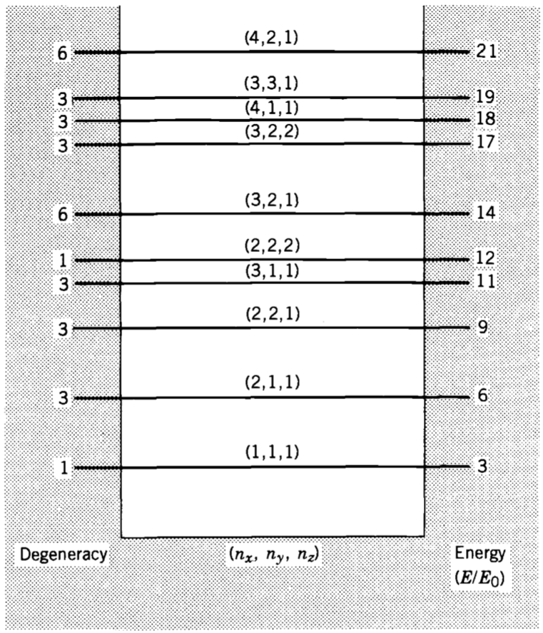
3D Infinite Square Well
The figure shows the energy levels of a particle confined to a 3D cubic box. The energy is given in units of \(E_0 = \dfrac{\hbar^2\pi^2}{2 m L^2}\).
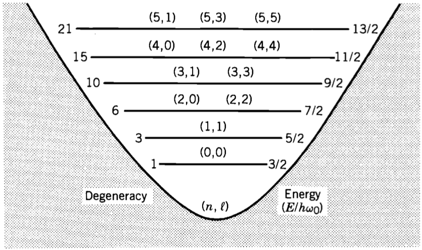
3D Isotropic Harmonic Potential Well
The figure shows some of the lower energy levels of a particle in a central 3D isotropic harmonic oscillator potential.
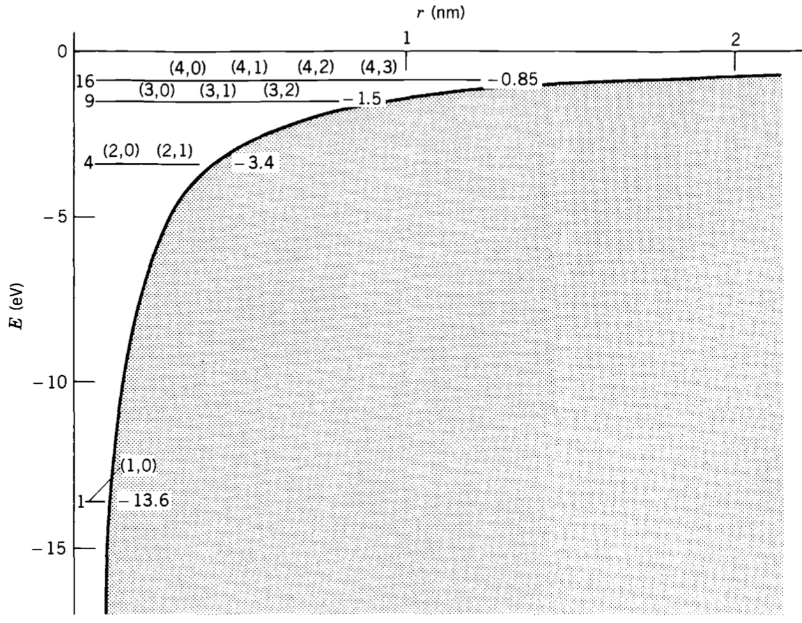
Coulomb Potential
The figure shows the lower energy levels in a Coulomb potential, shown for \(Z=1\) (hydrogen atom). The states are labelled with \((n,\ell)\); the degeneracies are indicated on the left and the energy values on the right.
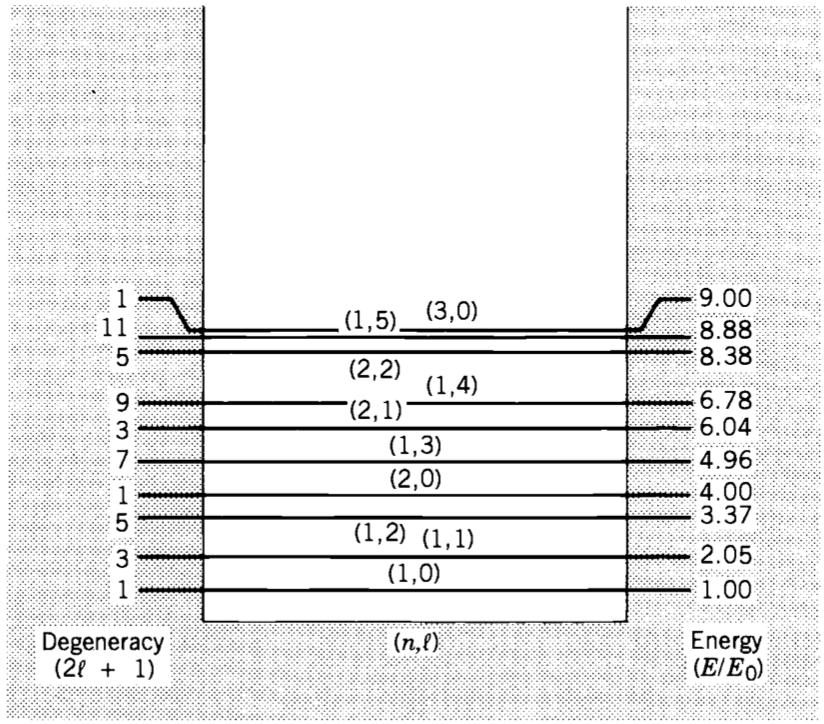
3D Infinite Spherical Well
Energy levels of a particle confined to a 3D spherical container. The energy is given in units of \(E_n = \dfrac{\hbar^2\pi^2}{2 m R^2}\). Note that the quantum number \(n\) does not arise directly in the solution in this case; it just serves to label(number) the states of a given \(\ell\).