15 Modelling the Nucleus III: The Shell Model
\[ \newcommand\v[1]{\boldsymbol{#1}} \newcommand\vdot[2]{\v{#1}\cdot\v{#2}} \]
\[ \newcommand{\dd}[2][]{\mathrm{d}^{#1}#2} \]
\[ \newcommand\f[2]{\dfrac{#1}{#2}} \newcommand\da[2]{\dfrac{d #1}{d #2}} \newcommand\daa[2]{\dfrac{d^2 #1}{d #2^2}} \newcommand\pa[2]{\dfrac{\partial #1}{\partial #2}} \newcommand\pal[3]{\left.\dfrac{\partial #1}{\partial #2}\right|_{#3}} \newcommand\paa[2]{\dfrac{\partial^2 #1}{\partial #2^2}} \newcommand\pab[3]{\dfrac{\partial^2 #1}{\partial #2 \partial #3}} \def\half{\frac{1}{2}} \]
\[ \newcommand\ket[1]{\left|#1\right\rangle} % |x> \newcommand\exp[1]{\left\langle#1\right\rangle} % <x> \newcommand\lr[1]{\left(#1\right)} % (x) \newcommand\lrs[1]{\left[#1\right]} % [x] \newcommand\lra[1]{\left|#1\right|} % |x| \newcommand\lrc[1]{\left\{#1\right\}} % {x} \newcommand\lrl[3]{\left.#1\right|_{#2}^{#3}} % x_limits \]
\[ \def\ie{\text{i.e.}\quad} \]
\[ \newcommand{\me}[3][\rightarrow]{{#2}#1{#3}} % Typical reaction \newcommand{\nr}[3]{{#1}\,({#2})\,{#3}} % Nuclear reactions \newcommand{\ele}[4]{_{#2}^{#3}{\textbf{#1}}_{#4}} \newcommand{\el}[2]{^{#2}\text{#1}} \newcommand{\til}[2][\mathbf{\sim}]{\underset{#1}{{#2}}} \newcommand{\b}[1]{\overline{#1}} \]
\[ \newcommand{\coulomb}[1]{\dfrac{#1}{4\pi\epsilon_0}} \def\degree{^*} \]
\[ \def\amu{\text{ amu}} \def\J{\text{ J}} \def\K{\text{ K}} \def\s{\text{ s}} \def\second{\text{ s}} \def\Psecond{\text{ s}^{-1}} \def\m{\text{ m}} \def\mm{\text{ mm}} \def\km{\text{ km}} \def\fm{\text{ fm}} \def\mum{\text{ $\mu$m}} \def\mus{\text{ $\mu$s}} \def\mPERs{\text{ ms$^{-1}$}} \def\eV{\text{ eV}} \def\keV{\text{ keV}} \def\GeV{\text{ GeV}} \def\MeV{\text{ MeV}} \def\MeVc{\text{ MeV/c$^2$}} \def\KeVc{\text{ KeV/c$^2$}} \newcommand\ttp[1]{\times 10^{#1}} % To The Power \]
\[ \def\en{\nu_e} \def\Aen{\b{\nu_e}} \def\mun{\nu_\mu} \def\Amun{\b{\nu}_\mu} \]
\[ \def\uraniumA{\ele{U}{92}{233}{}} \def\uraniumB{\ele{U}{92}{235}{}} \def\uraniumC{\ele{U}{92}{238}{}} \def\carbonB{\ele{C}{6}{14}{}} \def\nitrogenB{\ele{N}{7}{14}{}} \def\oxygenA{\ele{O}{8}{14}{}} \def\oxygenB{\ele{O}{8}{16}{}} \]
\[ % \def\com{\text{\scriptsize CM}} \def\com{\mathrm{\scriptsize CM}} \]
\[ \def\l{l} \]
\[ \def\g{\gamma} \]
What to Expect in This Chapter
I introduced nuclear magic numbers in Chapter 12 and noted that nuclei with magic numbers of protons or neutrons have distinctive properties. In this chapter, I will expand on these properties and take a first look at the nuclear Shell Model.
The Shell Model is important because it was the first successful model to explain how the magic numbers arise. Maria Goeppert Mayer and Johannes Jensen received the 1963 Nobel Prize in Physics for their work on the Shell Model.
15.1 Nuclear Magic
Although \(B/A\) follows a smooth trend on a broad scale, a careful examination of nuclear data reveals special values of the proton or neutron number:
\[ Z\text{ or }N = 2,\ 8,\ 20,\ 28,\ 50,\ 82,\ 126. \tag{15.1}\]
These are called magic numbers, and nuclei with a magic value of \(Z\) or \(N\) are called magic nuclei. Nuclei in which both \(Z\) and \(N\) are magic are called doubly magic nuclei.
These magic numbers are reminiscent of the electron-shell structure of atoms. In both cases, certain numbers of particles complete particularly stable configurations. Here, however, we are dealing with protons and neutrons within the nucleus, rather than electrons surrounding an atom.
Magic nuclei have several distinctive properties:
- They tend to have relatively large proton or neutron separation energies.
- They often have low neutron-capture cross-sections.
- They tend to have high energies for their first excited states.
- Closed-shell nuclei are usually spherical and have small electric quadrupole moments.
- Nuclear radii and separation energies show sudden changes near magic numbers.
15.1.1 Evidence for Magic Properties
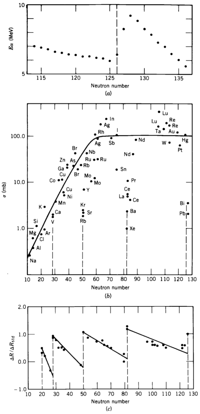
Figure Figure 15.1 shows several examples of the effect of magic numbers.
Figure (a) shows the energies of \(\alpha\) particles emitted by isotopes of \(\mathrm{Rn}\). Notice the sudden increase when the daughter nucleus has \(N=126\), which occurs when the parent nucleus has \(N=128\). A more tightly bound daughter nucleus allows the \(\alpha\) decay to release more energy.
Figure (b) shows neutron-capture cross-sections for various nuclei. Notice the decreases by roughly two orders of magnitude near \(N=50\), \(82\), and \(126\). A closed neutron shell makes it more difficult for the nucleus to capture an additional neutron.
Figure (c) shows the change in nuclear charge radius with \(\Delta N=2\). Notice the sudden changes near \(N=20\), \(28\), \(50\), \(82\), and \(126\). The radius difference \(\Delta R\) has been divided by the standard radius \(R\propto A^{1/3}\) in order to emphasise the shell effects.
15.2 The Shell Model
You will recall that solving the Schrödinger equation for the Coulomb potential of hydrogen naturally leads to atomic shells. Similarly, we might expect nuclear shells to emerge from a solution of the Schrödinger equation for nucleons in a nuclear potential.
However, we immediately encounter a difficulty. In an atom, electrons move in the well-known Coulomb potential created by the nucleus. In a nucleus, each nucleon interacts strongly with many other nucleons, and we do not know the exact form of the resulting potential.
As in the Fermi Gas Model, we therefore make a mean-field approximation: each nucleon moves independently in an average potential created by all the other nucleons.
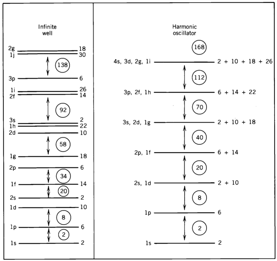
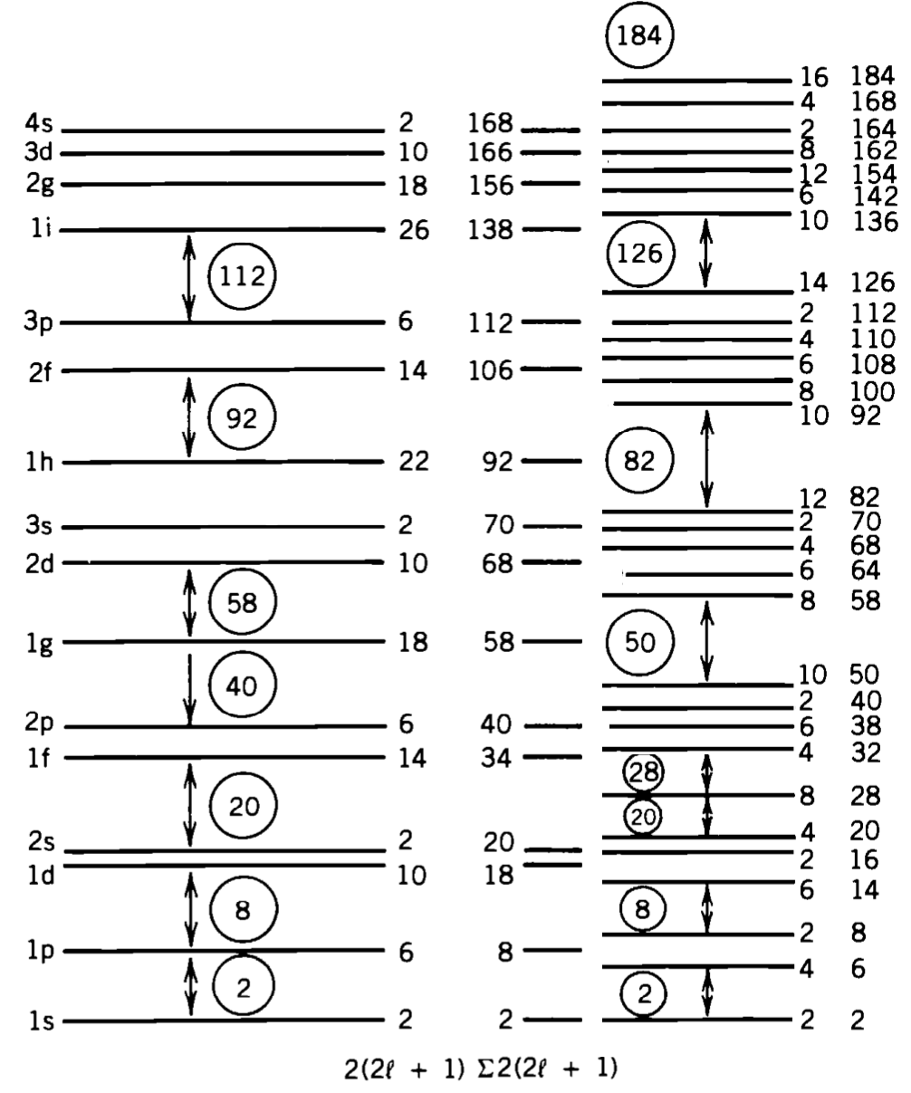
To get started, let us consider two simple potentials: the three-dimensional infinite spherical well and the three-dimensional isotropic harmonic oscillator. Figure Figure 15.2 shows the energy levels predicted by these potentials.
The number to the right of each level gives its capacity, including spin degeneracy. The circled numbers give the total number of nucleons when a shell is filled. Large gaps between energy levels indicate shell closures.
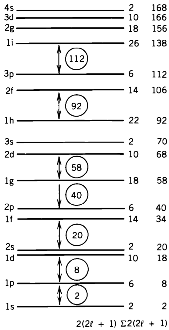
Neither of these simple potentials reproduces all the observed magic numbers. They account for \(2\), \(8\), and \(20\), but not for \(28\), \(50\), \(82\), or \(126\). This tells us that an important physical ingredient is missing.
15.3 A Better Potential
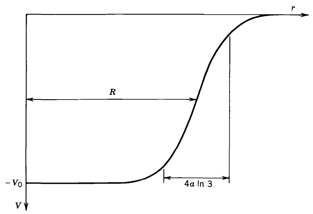
A more realistic mean-field potential is the Woods–Saxon potential, shown in Figure 15.4:
\[ V(r) = -\f{V_0}{1+e^{(r-R)/a}}. \tag{15.2}\]
Unlike a square well, the Woods–Saxon potential changes smoothly from a roughly constant value in the interior to zero outside the nucleus. It is therefore more realistic for a finite nucleus.
The parameter \(R\) is related to the nuclear radius, while \(a\) describes how quickly the potential changes at the nuclear surface. The surface thickness is commonly written as
\[ t=4a\ln3. \tag{15.3}\]
Typical parameter values are shown below.
| Parameter | Value |
|---|---|
| \(V_0\) | \(50\) MeV |
| \(R\) | \(1.25A^{1/3}\) |
| \(a\) | \(0.524\) fm |
Unfortunately, even the Woods–Saxon potential does not reproduce all the observed magic numbers, as shown in Figure 15.3.
15.4 Spin–Orbit Coupling of Nucleons
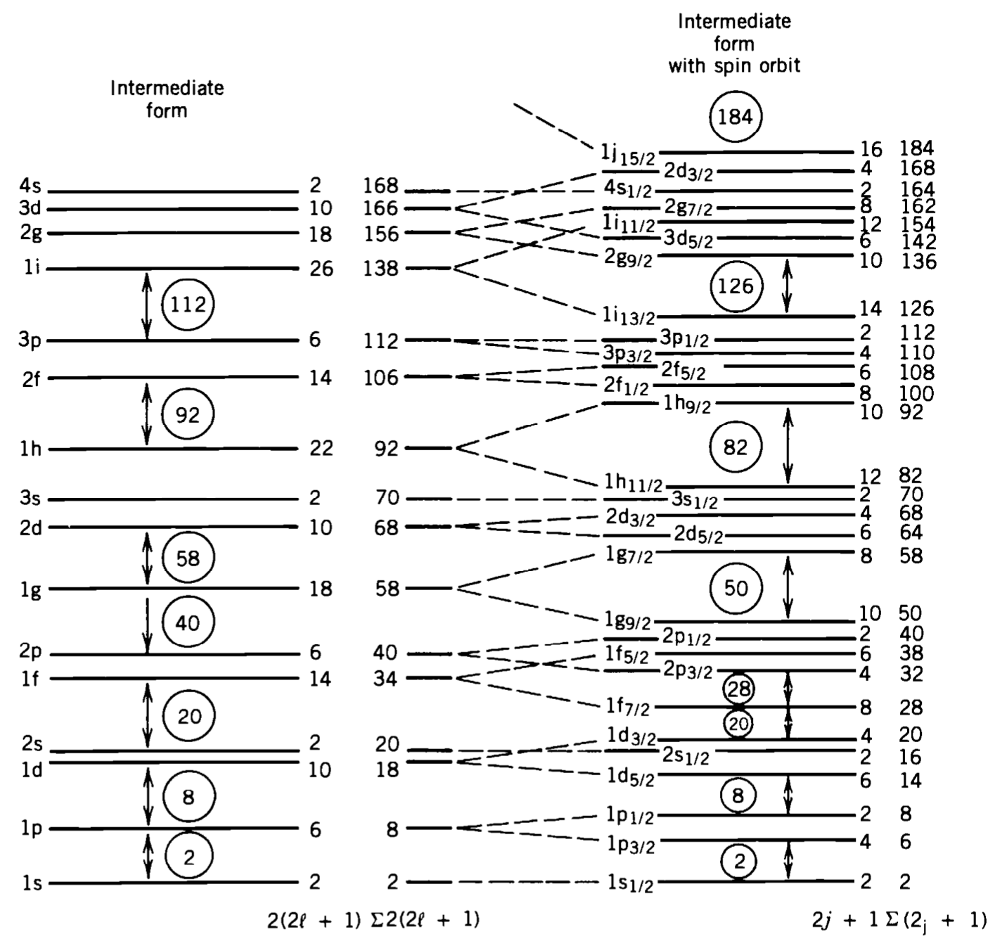
After about a decade without success, Mayer and Jensen reproduced all the observed magic numbers by introducing an additional term into the Woods–Saxon potential. As shown in Figure 15.5, this term rearranges the levels in exactly the way needed to produce the magic numbers.
Inspired by the fine-structure interaction in atomic physics, they included a nuclear spin–orbit interaction of the form
\[ V_{\mathrm{SO}}(r)\,\v{L}\cdot\v{S}. \tag{15.4}\]
Here, \(V_{\mathrm{SO}}(r)\) is a radial function whose strength is determined from nuclear data.
The orbital angular momentum \(\v{L}\) and intrinsic spin \(\v{S}\) couple to form the total angular momentum of a nucleon:
\[ \v{J} = \v{L}+\v{S}. \tag{15.5}\]
For a nucleon, \(s=\half\). The allowed values of \(j\) are therefore
\[ j = \ell\pm\frac{1}{2}. \tag{15.6}\]
Thus, except when \(\ell=0\), each orbital level splits into a pair of states called a spin–orbit doublet.
Although the directions of \(\v{L}\) and \(\v{S}\) are no longer separately fixed, the quantities \(L^2\), \(S^2\), \(J^2\), and \(J_z\) remain good quantum numbers. We can therefore label a single-particle state using \(n\), \(\ell\), \(j\), and \(m_j\).
To determine the splitting, note that
\[ \begin{align} \v{J}^2 &= (\v{L}+\v{S})^2 \\ &= \v{L}^2 + 2\v{L}\cdot\v{S} + \v{S}^2. \end{align} \]
Hence,
\[ \v{L}\cdot\v{S} = \f{1}{2} \lr{ \v{J}^2-\v{L}^2-\v{S}^2 }. \tag{15.7}\]
Taking the expectation value in a state of definite \(\ell\), \(s\), and \(j\) gives
\[ \exp{\v{L}\cdot\v{S}} = \f{1}{2} \lrs{ j(j+1)-\ell(\ell+1)-s(s+1) } \hbar^2. \tag{15.8}\]
For a nucleon, \(s=\half\). Therefore,
\[ \begin{align} \exp{\v{L}\cdot\v{S}}_{j=\ell+\frac{1}{2}} &= \f{1}{2}\ell\hbar^2,\\ \exp{\v{L}\cdot\v{S}}_{j=\ell-\frac{1}{2}} &= -\f{1}{2}(\ell+1)\hbar^2. \end{align} \tag{15.9}\]
The difference between the two values is
\[ \exp{\v{L}\cdot\v{S}}_{j=\ell+\frac{1}{2}} - \exp{\v{L}\cdot\v{S}}_{j=\ell-\frac{1}{2}} = \f{1}{2}(2\ell+1)\hbar^2. \tag{15.10}\]
The splitting therefore becomes larger as \(\ell\) increases.
For nuclei, the spin–orbit interaction has the sign required to push the \(j=\ell+\frac{1}{2}\) state down in energy relative to the \(j=\ell-\frac{1}{2}\) state. This large rearrangement of levels is the crucial feature that produces the magic numbers
\[ 2,\ 8,\ 20,\ 28,\ 50,\ 82,\ 126. \]
15.5 Angular Momentum of the Nucleus (\(\boldsymbol{I}\))
The total angular momentum of a nucleus is called its nuclear spin and is denoted by \(\v{I}\). It is made up of the orbital and intrinsic-spin angular momenta of all the nucleons:
\[ \v{I} = \sum_{i=1}^{A}\v{J}_i, \tag{15.11}\]
where
\[ \v{J}_i = \v{L}_i+\v{S}_i \tag{15.12}\]
is the total angular momentum of nucleon \(i\).
Since each nucleon has \(s_i=\half\), its possible total angular-momentum quantum numbers are
\[ \begin{align} j_i &= |\ell_i-s_i|,\ldots,\ell_i+s_i\\ &= \ell_i\pm\half. \end{align} \tag{15.13}\]
Because \(\ell_i\) is always an integer, each individual nucleon has half-integer \(j_i\).
15.5.1 \(jj\) versus \(LS\) Coupling
We construct the total angular momentum of the nucleus by adding the total angular momenta of the individual nucleons:
\[ \v{I} = \sum_i\v{J}_i, \qquad \v{J}_i=\v{L}_i+\v{S}_i. \tag{15.14}\]
This is called \(jj\) coupling.
An alternative is \(LS\) coupling, in which we first add all the orbital angular momenta to obtain \(\v{L}\), then add all the intrinsic spins to obtain \(\v{S}\), and finally combine \(\v{L}\) and \(\v{S}\) to obtain \(\v{I}\).
The \(jj\) coupling scheme is more appropriate for many nuclei because the spin–orbit interaction of each nucleon is strong. This is the same interaction that was essential for reproducing the observed magic numbers.
15.5.2 Trends in \(I\)
Let us first consider a nucleus with two nucleons. Since both \(j_1\) and \(j_2\) are half-integers, their combined angular momentum can take the values
\[ I = |j_1-j_2|,\ldots,j_1+j_2. \tag{15.15}\]
These values are always integers. More generally,
\[ I = \begin{cases} \text{integer}, & \text{for even $A$},\\ \text{half-integer}, & \text{for odd $A$}. \end{cases} \tag{15.16}\]
Further trends are seen in measured nuclear spins:
Ground states of even-even nuclei have \(I=0\). This indicates that protons and neutrons pair separately, with each pair contributing zero total angular momentum.
For odd-\(A\) nuclei, \(I\) is often relatively small. In many cases, the nuclear spin is determined mainly by the one unpaired proton or neutron.
When both \(Z\) and \(N\) are odd, the total angular momentum is determined by coupling the unpaired proton and unpaired neutron:
\[ \v{I} = \v{J}_p+\v{J}_n. \tag{15.17}\]
The possible values are
\[ I = |j_p-j_n|,\ldots,j_p+j_n. \tag{15.18}\]
15.6 Parity of the Nucleus
The parity of a nuclear state is obtained by multiplying the spatial parities of all its nucleons. Both the proton and neutron have positive intrinsic parity, so a nucleon in an orbital with angular momentum \(\ell_i\) contributes a spatial parity
\[ (-1)^{\ell_i}. \]
Thus, in general,
\[ \eta = \prod_i(-1)^{\ell_i}. \tag{15.19}\]
A pair of nucleons in the same orbital contributes
\[ (-1)^\ell(-1)^\ell=+1. \]
Thus, filled shells do not affect the overall parity. The parity is determined by the unpaired nucleons:
\[ \eta = \begin{cases} +1, & \text{even-even nuclei},\\ (-1)^{\ell}, & \text{odd-$A$ nuclei},\\ (-1)^{\ell_p}(-1)^{\ell_n}, & \text{odd-odd nuclei}. \end{cases} \tag{15.20}\]
15.7 Predicting Spin and Parity
The Shell Model can be used to predict the ground-state spin and parity of nuclei. It does a remarkably good job, although it is not perfect. The predictions depend on whether \(Z\) and \(N\) are even or odd.
15.7.1 Even-Even Nuclei
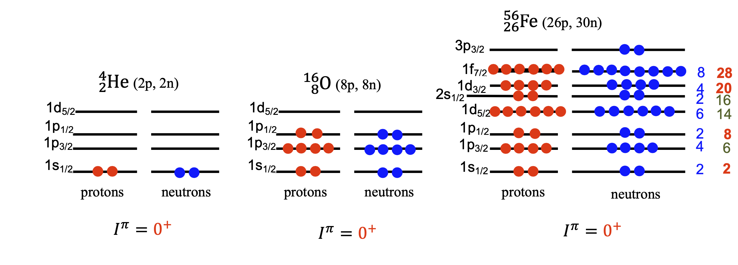
Examples of even-even nuclei include \({}^{4}\mathrm{H}\), \({}^{16}\mathrm{O}\), \({}^{56}\mathrm{Fe}\), and \({}^{238}\mathrm{U}\).
The Shell Model predicts that nucleons fill the available states from the bottom upwards. Because the protons and neutrons are separately paired, their angular momenta cancel. The ground-state nuclear spin is therefore
\[ I=0. \]
From Equation 15.20, the parity is positive. Thus, even-even nuclei have ground states with
\[ I^\eta=0^+. \tag{15.21}\]
There are no known exceptions to this rule for ground states.
15.7.2 Odd \(A\)
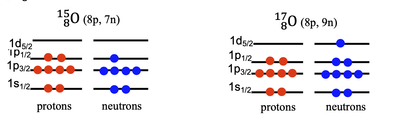
Examples of odd-\(A\) nuclei are \({}^{15}\mathrm{O}\) and \({}^{17}\mathrm{O}\). In these nuclei, the unpaired nucleon, determines the spin and parity of the ground state.
For \({}^{15}\mathrm{O}\), the relevant configuration is a neutron hole in a \(p_{1/2}\) orbital. Thus,
\[ {}^{15}\mathrm{O} \rightarrow \half^-. \]
For \({}^{17}\mathrm{O}\), the extra neutron occupies a \(d_{5/2}\) orbital. Thus,
\[ {}^{17}\mathrm{O} \rightarrow \frac{5}{2}^+. \]
The Shell Model agrees with the observed spin-parity assignments for most odd-\(A\) nuclei. There are, however, exceptions. For example, the simple shell model predicts \(\frac{5}{2}^+\) for \({}^{24}\mathrm{Na}\), whereas the measured value is \(\frac{3}{2}^+\).
15.7.3 Odd-Odd Nuclei
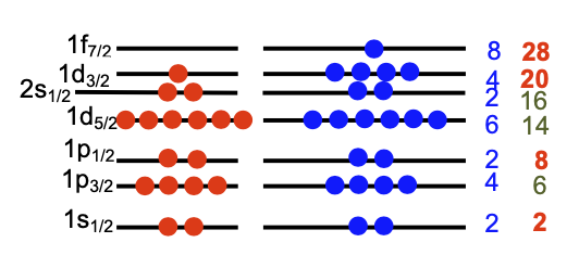
Let us consider \(\ele{Cl}{17}{38}{21}\) as an example. The total spin is due to the unpaired proton and unpaired neutron.
First, the parity is
\[ \eta = (-1)^2(-1)^3 = -1. \tag{15.22}\]
The proton and neutron have
\[ j_p=\frac{3}{2}, \qquad j_n=\frac{7}{2}. \]
Therefore, the possible total angular momenta are
\[ \left| \frac{7}{2}-\frac{3}{2} \right| \leq I \leq \frac{7}{2}+\frac{3}{2}. \tag{15.23}\]
Hence,
\[ I^\eta = 2^-, \ 3^-, \ 4^-, \text{ or } 5^-. \tag{15.24}\]
15.8 Beyond the Shell Model
The Shell Model is a major improvement over the Fermi Gas Model because it uses a more realistic mean-field potential and includes the strong spin–orbit interaction. It correctly reproduces all the observed magic numbers and can make good predictions of nuclear ground-state spin and parity.
However, the simple independent-particle Shell Model is incomplete. It has limited success in describing many excited states, magnetic moments, and strongly deformed nuclei. In particular, many nuclei have appreciable quadrupole moments, showing that their charge distributions are not spherical.
These observations motivated more sophisticated approaches, including collective and deformed-nucleus models. I will not discuss these models here. If you are interested, see Chapter 4 of1.