4 Discovering Stuff

What to expect in this chapter

In a previous chapter on particle physics, I introduced you to our current understanding of particle physics. We discussed leptons and quarks, flavours, gauge bosons, and the various quantum numbers $(L_e, L_\mu, L_\tau, D, U, S\ldots)$ used to describe these particles. In this chapter, I would like to discuss how we came about this knowledge.

Although the content of this chapter might feel historical, it highlights fundamental ideas that are necessary for you to make sense of nuclear reactions. It also features the bold and ingenious strategies, insights that physicists used to solve seemingly intractable problems.

4.1 Particle tracks

Before the particle accelerator at Brookhaven (called the Cosmotron) started working in 1952, most particle physics experiments relied on cosmic rays as a source of particles and cloud chambers and photographic emulsions as detectors. These detectors relied on the charge of the particles to create tracks in the detector, much like the contrails of an aeroplane. Let us quickly look at a few of these results to get a feel for what the pioneers of this field did and how it influenced the development of an overarching theory.

4.1.1 Particle tracks in a magnetic field

Since magnetic fields cause particle tracks to curve in a predictable fashion, they can be used to identify the properties of charged particles. For instance, the radius of curvature of the track is directly proportional to the particle’s speed. We can understand this by noting that if there is a change in speed, the Lorentz force ($q\v{v}\times\v{B}$) responsible for the curved motion changes in proportion to $v$, while the demands of the centripetal force vary as $v^2$. This means:

We can see this mathematically by:

\[\begin{align*} |q(\overrightarrow{v}\times \overrightarrow{B})| &=m\;\dfrac{v^{2}}{r}\\ \text{i.e. } qvB&=\dfrac{mv^{2}}{r}\\ \Rightarrow r&=\dfrac{mv}{qB}=\dfrac{v}{\left( q/m\right) B} \end{align*}\]

One trick that experimentalists used (for example, in discovering the electron) was to use an electric field to counter the effects of the magnetic field. In such a situation

\[qE=qbB\Rightarrow v=\dfrac{E}{B}\]

Whence,

\[r=\dfrac{1}{(q/m)}\left(\dfrac{E}{B^{2}}\right)\]

Thus, measuring the radius (along with the values of $E$ and $B$) can lead to the particle’s charge-to-mass ratio ($q/m$).

4.1.2 Sample Tracks

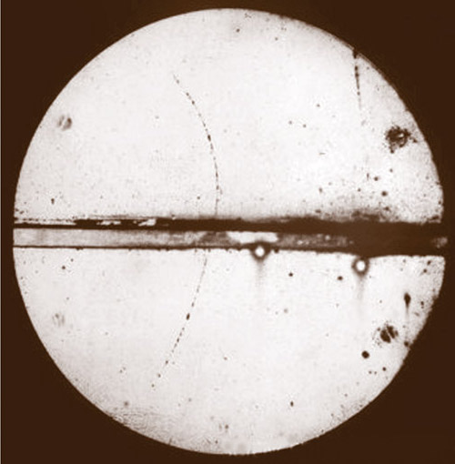
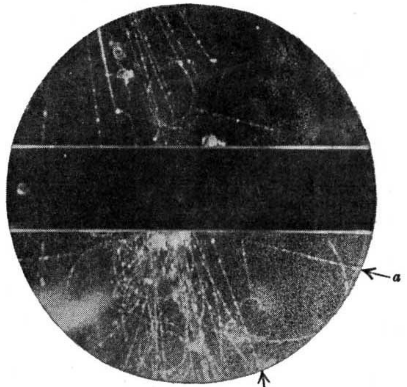
(a) Track made by a positron in a cloud chamber in the experiment conducted by Carl Anderson.

Figure 4.1 (a) shows the cloud chamber tracks Carl Anderson used to discover the positron. A magnetic field (going into the page) bends the trajectories of any charged particle. However, we cannot say if the track in the figure corresponds to a negatively charged particle moving downwards or a positively charged particle moving upwards. To distinguish between the two, the experimentalists placed a lead plate (the horizontal line) to slow the particle. When this happens, the radius of curvature of the path should decrease on the slower slide.

Figure 4.1 (b) shows the discovery of the first (strange) meson called the kaon ($K^0$). This uncharged particle does not show a track until it decays into a $\pi^\pm$ pair indicated by the ‘V’-shaped trajectories. \[ \me{K^0}{\pi^++\pi^-} \tag{4.1}\]

This discovery was startling because indications were that it was much heavier $(\approx 500 \MeV)$ than two pions $(\approx 2\times 140 \MeV)$. There was also something strange about them $\ldots$ (more about this later).

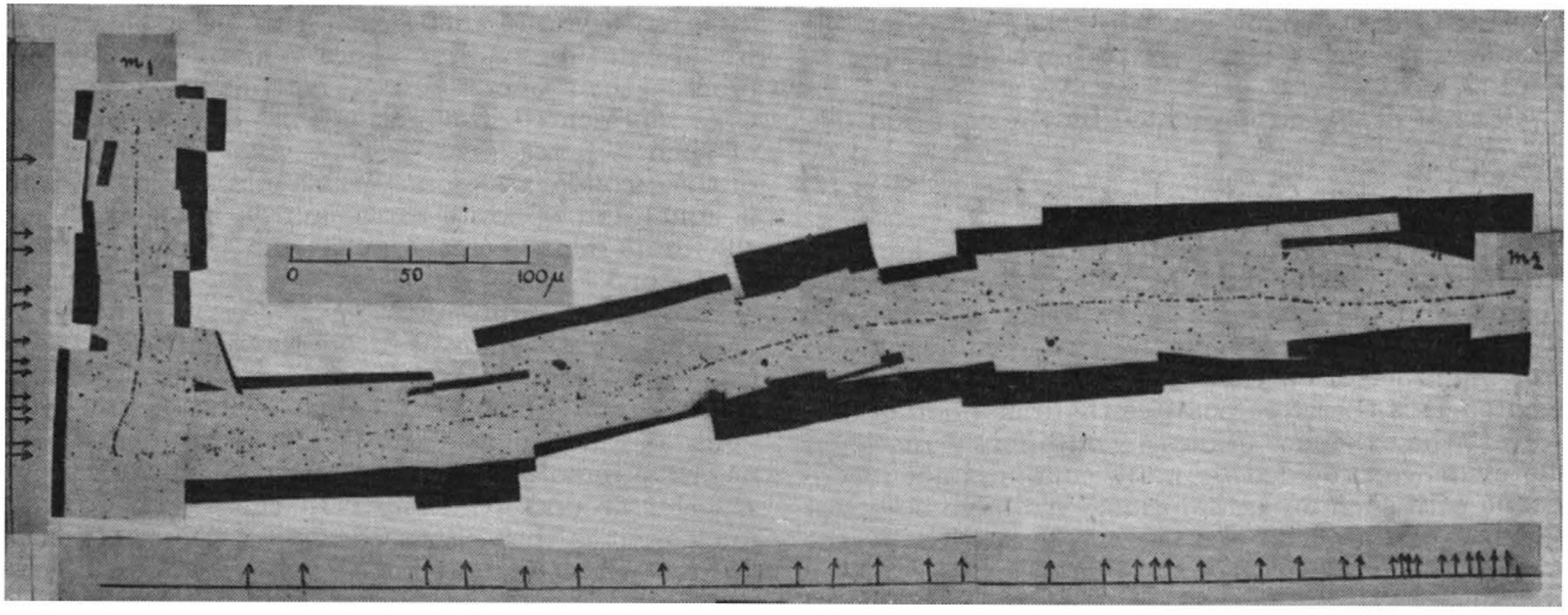
(a) Tracks in photographic emulsion left by a pion entering from the top left.

Figure 4.2 (a) shows a charged pion ($\pi^-$) entering from the top left and first decaying into a muon ($\mu^-$) and a neutrino ($\Amun$):

\[\me{\pi^-}{\mu^-+\Amun}\]

The abrupt changes in trajectories, without ‘anyone’ taking the momentum away in the opposite direction, made people suspect the existence of an ‘invisible’ particle, which we know today to be one of the neutrinos.

I like to share another example just to further highlight a few points. Figure 4.2 also shows the decay of a pion as in Figure 4.2 (a). However, it also shows the subsequent decay of the muon($\mu^{-}$). As with the pion decay, there are ‘invisible’ particles at play in the muon decay. However, there is a crucial difference: The data indicates that the muon always has the same energy, but the electron’s energy varies! So, by virtue of Equation 2.18 there must be one ‘invisible’ particle associated with the former decay and at least two associated with the latter. We now know that the reaction is given by:

\[ \me{\mu^-}{e^-+\Aen+\mun} \tag{4.2}\]

4.2 Getting Comfortable with Conservation

In Section 1.6.1 of the previous chapter, I introduced several quantum numbers and associated conservation laws. Here they are again:

Some conserved quantities
Always Conserved	Conserved When No Weak Interaction
Energy	Downness ($D$)
Linear and angular momentum	Upness ($U$)
Electric charge ($Q$)	Strangeness ($S$)
Electron number ($L_e$)	Charmness ($C$)
Muon number ($L_\mu$)	Bottomness ($B$)
Tau number ($L_\tau$)	Topness ($T$)
Baryon number ($A$)

In this section, I will show you how we discovered that these conserved quantities existed. But first, let’s get comfortable with using these laws.

Here are a few example particle reactions. I have indicated the various conserved numbers on the right. There are three instances where strangeness is not conserved because the decay happens through a weak interaction. In these cases, I have indicated the values of $S$ on either side.

In case you are wondering, Gell-Mann assigned $K$’s a strangeness of $+1$ and $\Sigma$’s and $\Lambda$ a strangeness of $-1$. The rest of the hadrons get a strangeness of $0$.

\[\begin{array}{clcrcll} \mee{1}{Anti proton production}{p+p}{p+p+p+p^{-}}{A=2} \mee{2}{Neutron decay}{n}{p^{+} + e^{-} + \Aen}{A=1, L_e=0} \mee{3}{Pair production}{\gamma}{e^{+} + e^{-}}{L_e=0} \mee{4}{$e^{-}$ -$e^{+}$ anhiliation}{e^{+} + e^{-}}{\gamma + \gamma}{L_e=0} \mee{5}{Muon decay}{\mu^{-}}{e^{-}+\Aen+\mun}{L_e=0, L_\mu=1} \mee{6}{Muon decay}{\mu^{+}}{e^{+}+\en+\Amun}{L_e=0, L_\mu=-1} \mee{7}{Pion decay}{\pi^{-}}{\mu^{-} + \Amun}{L_\mu=0} \mee{8}{Pion decay}{\pi^{+}}{\mu^{+} + \mun}{L_\mu=0} \mee{9}{Kaon production}{\pi^{-}+p^{+}}{K^{+}+\Sigma^{-}}{A=1, S=0} \mee{10}{Kaon decay}{K^{0}}{\pi^{+}+\pi^{-}}{S=1\neq S=0} \mee{11}{Kaon decay}{K^{+}}{\pi^{+}+\pi^{+}+\pi^{-}}{S=1 \neq S=0} \mee{12}{Baryon decay}{\Lambda^{0}}{p^{+}+\pi^{-}}{A=1, S=-1 \neq S=0} \end{array}\]

I have not included examples of other ‘nesses’ (e.g. charmeness) related to quarks. These work the same way as strageness.

4.3 Rules about Reactions

4.3.1 Somes rules

Now is a good time to look at some basic concepts related to particle interactions.

The first is called the principle of detailed balance. It say that if the following reaction is observed: \[\me{A+B}{C+D} \tag{4.3}\]

then it is also true that the reverse reaction should happen. i.e. this works too.

\[\me{C+D}{A+B} \tag{4.4}\]

The next principle is called principle of crossing symmetry and goes like this. If the following reaction is observed

\[\me{A+B}{C+D} \tag{4.5}\]

then, you will also ‘see’ the ones you get by swapping things about, provided that it is not forbidden by conservation of energy. What I mean by ‘swapping things’ is

\[ \begin{align} \me{A}{\b{B} + C+D} \\ \me{A+\b{C}}{\b{B}+D} \\ \me{\b{C}+\b{D}}{\b{A}+\b{B}} \\ \end{align} \tag{4.6}\]

Notice that you must convert the particle to the antiparticle if you cross it over.

4.3.2 Same, same but different

These ideas allow us to gain deeper insights into the processes that sometimes appear differently. For example, take Compton scattering:

\[ \gamma +e^{-}\rightarrow e^{-}+\gamma \tag{4.7}\]

Noting that the antiparticle of the photon is itself, we can rewrite this reaction as

\[ e^{-}+e^{+}\rightarrow \gamma +\gamma \tag{4.8}\]

However, this is electron-positron pair annihilation.

We could go farther;

\[ \gamma +\gamma \rightarrow e^{+}+e^{-} \tag{4.9}\]

This is pair production in free-space!

So, these processes are dynamically the same but are very different experimentally!

4.3.3 Feynman’s rule of thumb

There is an important rule of thumb in particle physics attributed to Richard Feynman:

Whatever is not explicitly forbidden is mandatory

This is significant because if we don’t observe certain reactions experimentally, it can indicate the presence of a deeper law of nature that forbids them. You will see several instances of this idea being put into use later.

4.4 We Need A Neutrino

4.4.1 Problems with $\beta$-decay

Before we go any further, we need to discuss the neutrino because some conservation laws pop out when we try to make sense of neutrinos. We know that the process of $\beta$-decay proceeds as follows.

\[ \me{n}{p^+ + e^- + \Aen} \tag{4.10}\]

However, in the 1930s, nobody knew about the neutrino, so (at that time) $\beta$-decay was known as.

\[ \me{n}{p^+ + e^-} \tag{4.11}\]

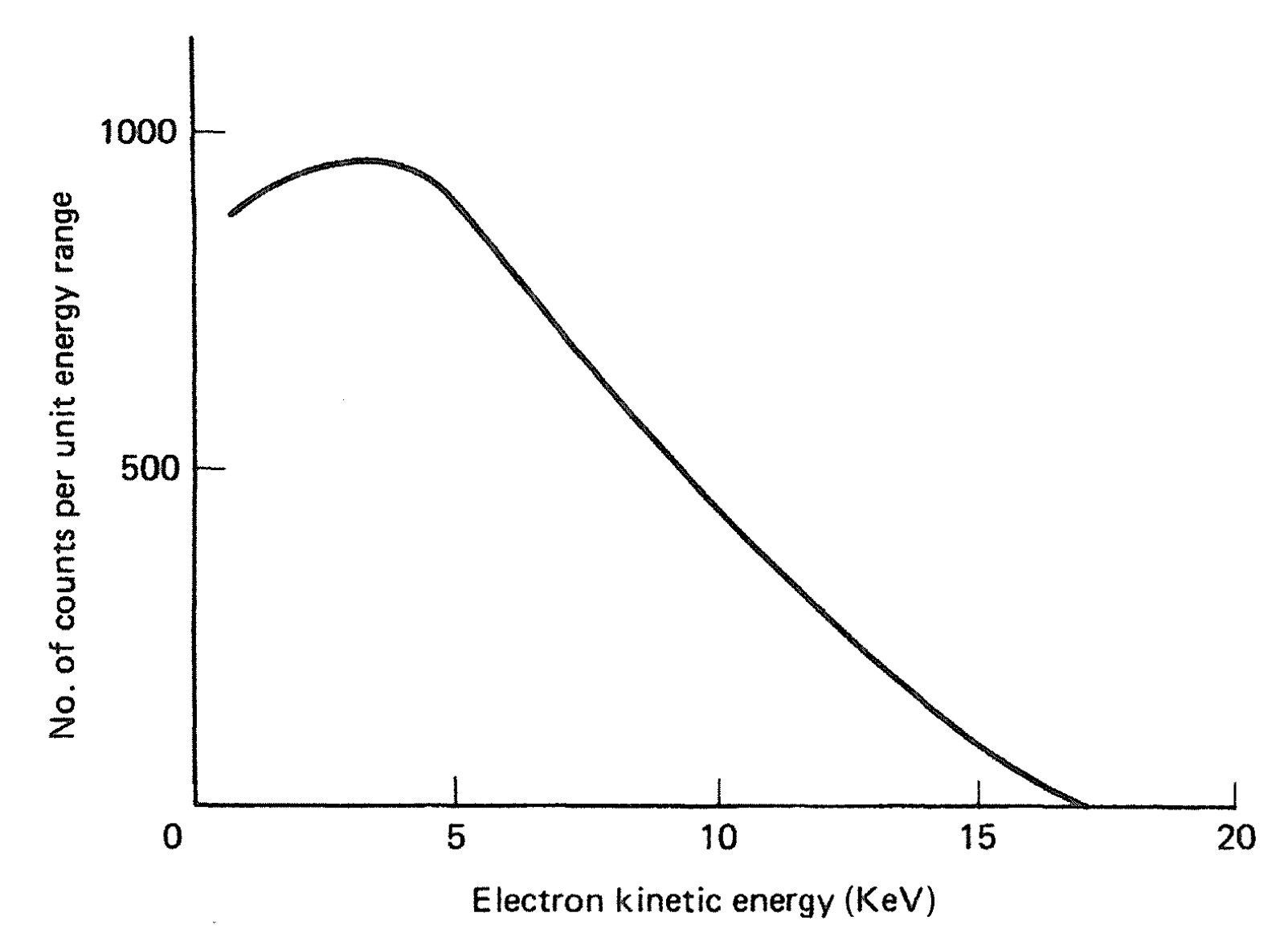
Figure 4.3: The energy of the exiting electron in the $\beta$-decay of tritium ($\me{\ele{H}{1}{3}{}}{\ele{He}{2}{3}{}}$)

Since this reaction has only two products, we know, by equation Equation 2.18, that the energy of the outgoing electron must be fixed. The experimental data for the $\beta$-decay of tritium ($\me{\ele{H}{1}{3}{}}{\ele{He}{2}{3}{}}$) showed a continuous energy spectrum for exiting electron as seen in figure Figure 4.3. This indicated that there were more than two products. Fermi called this extra particle the neutrino (‘little neutral one’) and used it in 1930 in his theory of $\beta$-decay.

Despite the success, people were still sceptical about the existence of the neutrino. So, in 1956 Cowan and Reines looked for confirmation by looking at the inverse beta decay reaction shown below. This is based on applying crossing symmetry to reaction Equation 4.10.

\[ \me{p^+ +\Aen}{n+ e^+} \tag{4.12}\]

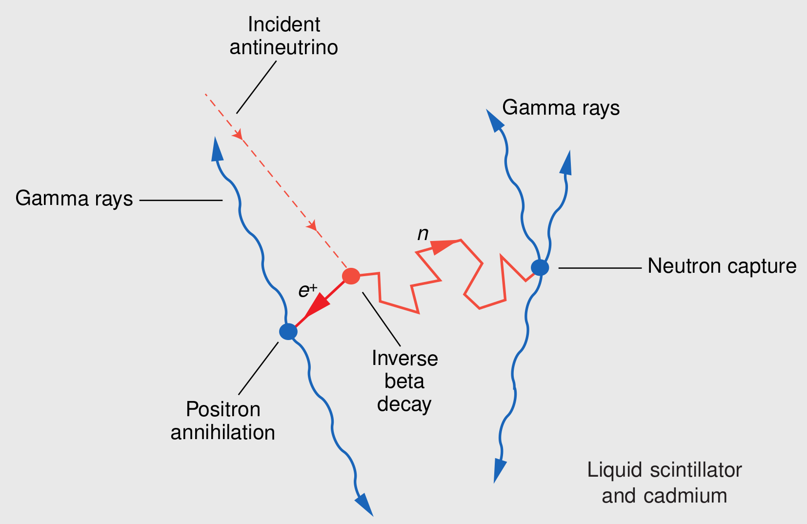
The experiment was set up (Figure 4.4) using 400 litres of water and multiple photomultiplier tubes to measure the pair of gamma rays produced by the subsequent annihilation of the positron ($\me{e^++e^-}{2\gamma}$). This technique is known as coincidence measurements, where we look for two photons at opposite ends that must trigger the photomultiplier tubes ‘simultaneously’. Additionally, $\text{CdCl}$ was also added to the water to enable the following reaction:

\[ \me{n + \ele{Cd}{}{108}{}}{\ele{Cd}{}{109}{} + \gamma} \]

However, the gamma from this reaction would be delayed by approximately $5\,\mu s$. So, the evidence for the reaction of equation Equation 4.12 was the coincident detection of a pair of gamma rays followed by another gamma $5\,\mu s$ later. This experiment confirmed the neutrino’s existence. Reines was awarded the Nobel Prize for this work in 1995 (Cowan had unfortunately already passed away).

4.4.2 Is there a difference between $\nu$ and $\b{\nu}$?

Since the neutrino carried no charge, people wondered if the neutrino and the antineutrino were the same (as with the photon or the neutral pion, $\pi^0$). To test this, Davis and Harmer argued that, following Cowan and Reines’ result, (using crossing symmetry)

\[ \me{\nu+n}{p^+ + e^-} \]

must occur. Further, if antineutrinos were no different from neutrinos, then the following should also happen:

\[ \me{\b{\nu}+n}{p^+ + e^-} \]

It was experimentally established that the former did occur and the latter did not. So, the neutrino and antineutrino are different particles. But what is the difference?

4.4.3 Hello Lepton Number

It was soon realised that all the known facts about neutrinos and antineutrinos can be reconciled if we introduce a Lepton number $L$, and a corresponding law of conservation of lepton number. With the inclusion of this lepton number, it was clear that certain processes, such as

\[ \me{\nu+n}{p^+ + e^-} \]

\[ \me{\b{\nu}+n}{p^+ + e^-} \]

would not work. So the ‘thing’ that makes a neutrino different from an antineutrino is the Lepton number!

4.4.4 One $L$ is not enough

There was still a problem because the following decay of a muon was never observed, but it was consistent with the conservation of $L$.

\[ \me{\mu^-}{e^-+\gamma} \]

Recalling Feynman’s rule of thumb about reactions, it was realised that there was more than one lepton number. Hence, $L_e, L_\mu$ and $L_\mu$ come into the picture. With their inclusion, it was clear why specific processes such as

\[ \me{\b{\nu}+n}{p^+ + e^-} \]

did not work. However, this meant that there was more than one type of neutrino! This was confirmed in 1962 by testing the reactions.

\[ \me{\Amun + p^+}{\mu^++n} \]

and

\[ \me{\Amun + p^+}{e^++n} \]

4.5 Quarks

4.5.1 Strangeness Descends

Around 1947, several startling discoveries in particle physics again demanded changes in our description of elementary particles. One was the discovery of the kaon ($K^0$, $K^+$) (see Figure 4.1 (b)) and the other was the lambda ($\Lambda$). The kaon was a meson and the $\Lambda$ had to be a baryon. They were observed to decay as:

\[ \left.\begin{align} &\me{K^0}{\pi^+ + \pi^-}\\ &\me{K^+}{\pi^+ + \pi^+ + \pi^-}\\ &\me{\Lambda}{p^+ + \pi^-} \end{align}\qquad\right \}\text{ Slow $\sim 10^{-10}$ s} \tag{4.13}\]

One of the surprising features was their large masses. Another was that these particles always appeared in pairs, showing up in reactions such as: \[ \left.\begin{align} \me[&\rightarrow]{\pi^-+p^+}{K^++\Sigma^-}\\ \me[&\rightarrow]{}{K^0+\Sigma^0}\\ \me[&\rightarrow]{}{K^0+\Lambda}\\ \end{align}\qquad\right \}\text{ Fast $\sim 10^{-23}$ s} \tag{4.14}\]

and never in reactions such as those shown below, despite them being consistent with all the rules known at that time.

\[ \left. \begin{align} \me[&\nrightarrow]{\pi^-+p^+}{\pi^++\Sigma^-}\\ \me[&\nrightarrow]{}{\pi^0+\Lambda}\\ \me[&\nrightarrow]{}{K^0+n}\\ \end{align}\qquad\right \}\text{ Not observed} \tag{4.15}\]

Another more revealing observation was that they were produced fast ($10^{-23}$) but decayed slowly ($10^{-10}$). Again, this indicated something new was at play. We now understand these observations by noting that the strong interaction produces these particles, while they decay via the weak interaction.

Gell-Mann and Nishijima realised that these observations were neatly explained if we introduce a new number called Strangeness ($S$) that is conserved during a strong interaction and not conserved during a weak interaction. The $K$’s were assigned a strangeness $S=+1$ and $\Sigma$’ and $\Lambda$’s, $S=-1$. The other particles do not have strangeness ($S=0$).

4.5.2 Prelude To Quarks - ‘The Eightfold Way’

Now let’s try to see how quarks came into the picture. The credit for the quark theory goes mostly to Murray Gell-Man, who is undoubtedly the Mendeleev of particle physics. In 1964, Gell-Mann attempted to bring order to the rapidly growing number of particles by organising them into various schemes. For example the Baryon Octet^‘Octet’ means ‘a group of eight’., Meson Octet(Figure 4.6) and the Baryon Decuplet^‘Decuplet’ means ‘a group of ten’.. He called these schemes the “Eightfold Way” (original article).

Source: Wikipedia

When Gell-Mann was putting these together, the $\Omega^-$ particle was unknown. So, in a Mendeleevian reenactment, Gell-Mann predicted its existence in 1961. He even predicted its mass and lifetime. The $\Omega^-$ was discovered in 1964, cementing the validity of the Eightfold Way. More particles were found afterwards, and they all fit into various other supermultiplets of the Eightfold Way. This categorisation is later extended to include the Charmness ($C$). I will not discuss these, but the idea is that all the particles fit into a neat categorisation scheme.

4.5.3 ‘Three Quarks For Master Mark’

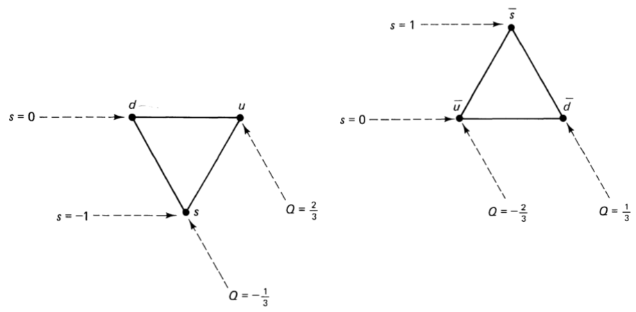
Gell-Mann and Zweig soon realised that the patterns observed in the Eightfold Way could be accounted for by assuming that hadrons were made up of three types (or “flavours”) of even more elementary particles: the up, down, and strange quarks. Gell-Mann used the term ‘quarks’ because they came as there were three, which reminded him of the phrase from ‘Three quarks for Master Mark’ from ‘Finnegans Wake’ by James Joyce.

Here are the diagrams for the three ($u$, $d$, $s$) quarks and antiquaks ($\b{u}, \b{d}, \b{s}$).

Figure 4.8: The $u$, $d$, and $s$ quarks in the Eightfold Way.

Making Baryons With Quarks

Here are the unique baryons we can create with the three $u$, $d$, and $s$ quarks in a combination of $qqq$.

Quark content	Q (Charge)	S (Strangeness)	Baryon
$uuu$	2	0	$\Delta^{++}$
$uud$	1	0	$\Delta^{+}$
$udd$	0	0	$\Delta^{0}$
$ddd$	-1	0	$\Delta^{-}$
$uus$	1	-1	$\Sigma^{*+}$
$uds$	0	-1	$\Sigma^{*0}$
$dds$	-1	-1	$\Sigma^{*-}$
$uss$	0	-2	$\Xi^{*0}$
$dss$	-1	-2	$\Xi^{*-}$
$sss$	-1	-3	$\Omega^{-1}$

Making Mesons With Quarks

Here are the unique mesons we can create with the three $u$, $d$, and $s$ quarks in a $q\b{q}$ pair.

Quark content	Q (Charge)	S (Strangeness)	Meson
$u\b{u}$	0	0	$\pi^{0}$
$u\b{d}$	1	0	$\pi^{+}$
$d\b{u}$	-1	0	$\pi^{-}$
$d\b{d}$	0	0	$\eta$
$u\b{s}$	1	1	$K^{+}$
$d\b{s}$	0	1	$K^{0}$
$s\b{u}$	-1	-1	$K^{-}$
$s\b{d}$	0	-1	$\b{K^{0}}$
$s\b{s}$	0	0	$\eta'$

Some Things To Take Note

There are a few things I would like to draw your attention to:

$\Sigma$ and $\Xi$ are different from $\Sigma^*$ and $\Xi^*$. The former belong to the spin $\frac{1}{2}$ Baryon octet, while the latter belong to the spin-$\frac{3}{2}$ Baryon decuplet.
In the table are nine combinations, but only eight particles in the Meson octet. This missing particle is the $\eta'$. Therefore, the Meson octet is really a Meson nonet¹.
Based on the above quark assignments, we cannot distinguish between $u\overline{u}$($\pi^0$), $d\overline{d}$($\eta$) and $s\overline{s}$($\eta'$). This is why the three particles are shown as the orthogonal combination of:

\[\begin{align} \pi^0 =& (u\overline{u}-d\overline{d})/\sqrt{2}\\ \eta =& (u\overline{u}+d\overline{d}-2s\overline{s})/\sqrt{6}\\ \eta' =& (u\overline{u}+d\overline{d}+s\overline{s})/\sqrt{3}\\ \end{align}\]

The antimesons automatically fit into the same nonet. For example, $\pi^+ = (u\overline{d})$ and $\pi^- = (d\overline{u})$.
Compare the quark content of $\Delta^+$ and $p$, and of $\pi^+$ and $\rho^+$. They are the same!
Our current understanding is that what we see here as different particles are excitation states of the same $uud$ and $u\overline{d}$ hadrons! In principle, each combination can spawn an infinite number of particles corresponding to excitation states.

4.5.4 The Charm Of The November Revolution

I won’t go into much detail here, but in 1974 a new extremely massive (approximately three times the mass of a proton) particle called the $\Psi$ (or $J$) was discovered. This led to what is known as the November Revolution, which ended with the introduction of a fourth quark called charm ($c$), which was experimentally verified in 1974. Similarly, a fifth quark, the bottom ($b$), was introduced after discovering the upsilon ($\Upsilon$) particle. At this point, no one was surprised that there should be a sixth quark, known as the top quark ($t$), considering there were six leptons. This was discovered in 1995.

4.5.5 Problems With The Quarks

Have You Seen A Quark?

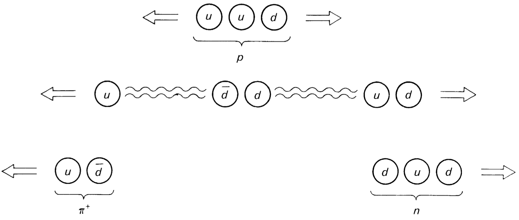
One of the main objections to the quark theory was that no one had experimentally observed quarks. However, there were deep inelastic scattering experiments at SLAC and CERN that showed that the proton had a ‘three lump’ structure. This led to the idea of quark confinement, which claimed that quarks are so strongly held by the strong force that they are absolutely confined. Pulling them apart required so much energy that you would create another particle instead. Figure Figure 4.9 shows a possible scenario for quark confinement.

Figure 4.9: A possible mechanism for quark confinement.

Hey, What About Pauli?

Another objection to the quark model was that it seemed to blatantly ignore Pauli’s Exclusion Principle, despite quarks being fermions. To fix this problem, Greenberg introduced the idea of colour to add more degrees of freedom. Although this initially seemed like a cheap trick, colour has turned out to be very useful. For example, since all naturally occurring particles must be colourless, this nicely explains why we don’t have elementary particles made of two or four quarks.

4.6 Theoretical Musings

Although I did not mention it so far, there was a parallel effort going on to understand particle physics theoretically.

4.6.1 Yukawa Theory

The first such theory was related to the strong force and was developed by Hideki Yukawa in 1935. He wanted to model the virtual force carrier of the strong force (called the Yukawa meson) and determine its mass. To do this, he used the energy-time uncertainty principle. The argument goes as follows.

The particle must carry the force across the size ($r_0$) of the nucleus. Assuming it was travelling very fast (close to the speed of light), the time it would take to cross the nucleus is $\Delta t =\dfrac{ r_0}{c}$. If it were to live that long, the energy ($\Delta E$) it can have without upsetting the energy-time principle is $\dfrac{\hbar c}{2 r_0}$.

If we take this as the rest mass ($\Delta E = mc^2$), then the mass of the Yukawa meson is given by:

\[ m = \dfrac{\hbar}{2 r_0\,c} \]

We now know that the mediator of the strong force is the massless gluon. However, the search for the Yukawa meson lead us to the muon ($\mu$), pion($\pi$).

4.6.2 Klein-Gorden And Dirac Equations

The start of quantum field theory can be traced back to the Klein-Gordon equation, which attempted to marry relativity with quantum mechanics. The equation was created by using the quatum operators for energy $\left(i\hbar\pa{}{t}\right)$ and momentum $\left(\dfrac{\hbar}{i}\nabla\right)$ in the relativistic equation $E^2 = p^2c^2 + m^2c^4$ which yielded:

\[ \left(\dfrac{1}{c^2}\paa{}{t} - \nabla^2 + \dfrac{m^2c^2}{\hbar^2}\right)\Psi = 0 \]

However, among the many problems of the Klein-Gordon equation was negative probabilities. Paul Dirac built on the Klein-Gordon equation by proposing and solving the Dirac equation:

\[ \left(i\hbar\pa{}{t} - i \alpha \cdot \nabla + \beta mc^2 \right)\Psi=0 \]

$\alpha$ and $\beta$ are four-component matrices called spinors.

Solving these equations is beyond what we can do in this module. However, I must add that both equations (theoretically!) demanded the existence of antiparticles. There were some issues of interpretation, but this was ironed out by Feynman and Stueckelberg. The discovery of the positron in 1931 was a major triumph for the theory.

4.6.3 Other Theories

In addition to quantum field theory predicting antiparticles, it also provided proof of the Exclusion Principle, the TCP theorem (related to how some processes violate time, charge, or parity symmetry), and proof of why spin-half particles are fermions. These theories, such as quantum-electrodynamics, quantum-chromodynamics, electroweak theory, Glasshow-Weinberg-Salam (GWS) theory, were developed by many people over many years. I will not attempt to discuss these here as I can only do so descriptively. You can learn about them in more advanced courses on field theory.

Chapter References

A nonet is a group of nine.↩︎

Always Conserved	Conserved When No Weak Interaction
Energy	Downness (\(D\))
Linear and angular momentum	Upness (\(U\))
Electric charge (\(Q\))	Strangeness (\(S\))
Electron number (\(L_e\))	Charmness (\(C\))
Muon number (\(L_\mu\))	Bottomness (\(B\))
Tau number (\(L_\tau\))	Topness (\(T\))
Baryon number (\(A\))

Quark content	Q (Charge)	S (Strangeness)	Baryon
\(uuu\)	2	0	\(\Delta^{++}\)
\(uud\)	1	0	\(\Delta^{+}\)
\(udd\)	0	0	\(\Delta^{0}\)
\(ddd\)	-1	0	\(\Delta^{-}\)
\(uus\)	1	-1	\(\Sigma^{*+}\)
\(uds\)	0	-1	\(\Sigma^{*0}\)
\(dds\)	-1	-1	\(\Sigma^{*-}\)
\(uss\)	0	-2	\(\Xi^{*0}\)
\(dss\)	-1	-2	\(\Xi^{*-}\)
\(sss\)	-1	-3	\(\Omega^{-1}\)

Quark content	Q (Charge)	S (Strangeness)	Meson
\(u\b{u}\)	0	0	\(\pi^{0}\)
\(u\b{d}\)	1	0	\(\pi^{+}\)
\(d\b{u}\)	-1	0	\(\pi^{-}\)
\(d\b{d}\)	0	0	\(\eta\)
\(u\b{s}\)	1	1	\(K^{+}\)
\(d\b{s}\)	0	1	\(K^{0}\)
\(s\b{u}\)	-1	-1	\(K^{-}\)
\(s\b{d}\)	0	-1	\(\b{K^{0}}\)
\(s\b{s}\)	0	0	\(\eta'\)

4 Discovering Stuff

What to expect in this chapter

4.1 Particle tracks

4.1.1 Particle tracks in a magnetic field

4.1.2 Sample Tracks

4.2 Getting Comfortable with Conservation

4.3 Rules about Reactions

4.3.1 Somes rules

4.3.2 Same, same but different

4.3.3 Feynman’s rule of thumb

4.4 We Need A Neutrino

4.4.1 Problems with \(\beta\)-decay

4.4.2 Is there a difference between \(\nu\) and \(\b{\nu}\)?

4.4.3 Hello Lepton Number

4.4.4 One \(L\) is not enough

4.5 Quarks

4.5.1 Strangeness Descends

4.5.2 Prelude To Quarks - ‘The Eightfold Way’

4.5.3 ‘Three Quarks For Master Mark’

Making Baryons With Quarks

Making Mesons With Quarks

Some Things To Take Note

4.5.4 The Charm Of The November Revolution

4.5.5 Problems With The Quarks

Have You Seen A Quark?

Hey, What About Pauli?

4.6 Theoretical Musings

4.6.1 Yukawa Theory

4.6.2 Klein-Gorden And Dirac Equations

4.6.3 Other Theories

Chapter References